Link to Lectures

Instructor: Prof. Michael Sipser

Book: “Introduction to the Theory of Computation” by Michael Sipser

ROUGH NOTES (!)
Updated: 8/2/24

Lec-1:

Computability Theory (1930s - 50s): What is computable or not ?

• Eg: Program verification, Pure mathematical truth
• Models of computation: Finite automata, Turing machines

Complexity Theory (1960s - Present): What is computable in practice ?

• Eg: Factoring problem, in fact P vs NP problem
• Measures of complexity: Time and Space

P vs NP is a millennium prize problem. Geometric Complexity Theory is a research program aimed at resolving this is.

A finite automaton is a ${ 5 - }$tuple ${ (Q, \Sigma, \delta, q _0, F) }$ where:

• ${ Q }$ is a finite set of states
• ${ \Sigma }$ is a finite set of alphabet symbols
• ${ \delta }$ is a transition function ${ \delta : Q \times \Sigma \to Q }$
• ${ q _0 \in Q }$ is the start state
• ${ F \subseteq Q }$ is the set of final/accept states.

A string is a finite sequence of symbols in ${ \Sigma }.$ A language is a (finite or infinite) set of strings.
The empty string ${ \varepsilon }$ is the string of length ${ 0 .}$ The empty language ${ \emptyset }$ is the language with no strings.

Finite automaton ${ M }$ accepts string ${ w = w _1 \ldots w _n }$ (each ${ w _i \in \Sigma }$) if there is a sequence of states ${ r _0, r _1, \ldots, r _n \in Q }$ such that:

• ${ r _0 = q _0 }$
• ${ r _i = \delta (r _{i-1}, w _i) }$ for ${ 1 \leq i \leq n }$
• ${ r _n \in F .}$

For a finite automaton ${ M ,}$ the language ${ L(M) = \lbrace w \vert M \text{ accepts } w \rbrace }$ is called the language of ${ M .}$ (We also say ${ M }$ recognizes ${ L(M) }$).
A language is called regular if some finite automaton recognizes it.

Goal: Understand the regular languages.

Eg: The language ${ \lbrace w \in \lbrace 0,1 \rbrace ^{*} \vert w \text{ contains substring } 11 \rbrace }$ is regular. (Language of the automaton here at 30:00).
The language ${ \lbrace w \vert w \text{ has equal number of } 0s \text{ and } 1s \rbrace }$ is not regular (will show later).

Operations on languages:
Let ${ A, B }$ be languages. Then we have languages:

• Union ${ A \cup B }$ ${ = \lbrace w \vert w \in A \text{ or } w \in B \rbrace }$
• Concatenation ${ AB }$ ${ = \lbrace xy \vert x \in A \text{ and } y \in B \rbrace }$
• Star ${ A ^{*} }$ ${ = \lbrace x _1 \ldots x _{k} \vert \text{each } x _i \in A \text{ for } k \geq 0 \rbrace }$ (Note empty string ${ \varepsilon \in A ^{*} }$ always).

We say ${ R }$ is a regular expression if ${ R }$ is:

• ${ a }$ for some ${ a \in \Sigma }$
• ${ \varepsilon }$
• ${ \emptyset }$
• ${ R _1 \cup R _2 }$ where ${ R _1, R _2 }$ are regular expressions
• ${ (R _1 \circ R _2) }$ where ${ R _1, R _2 }$ are regular expressions
• ${ R _1 ^{*} }$ where ${ R _1 }$ is a regular expression.

Informally, regular expressions are built from elements of ${ \Sigma ,}$ empty string ${ \varepsilon ,}$ empty set ${ \emptyset ,}$ and finite union, concatenation, star operations.

Eg: Say ${ \Sigma = \lbrace 0, 1 \rbrace. }$ Expression ${ (0 \cup 1) ^{*} = \Sigma ^{*} }$ gives all strings over ${ \Sigma = \lbrace 0, 1 \rbrace }.$ Expression ${ \Sigma ^{*} 1 }$ gives all strings that end in ${ 1 }.$ Expression ${ \Sigma ^{*} 1 1 \Sigma ^{*} }$ gives all strings that contain ${ 1 1 .}$ (These are regular languages, not a coincidence).

Goal: Show finite automata are equivalent to regular expressions.

We’ll show regular languages are closed under finite ${ \cup },$ ${ \circ }$ and ${ (\cdots) ^{*}. }$

Thm: If ${ A _1, A _2 }$ are regular languages, so is ${ A _1 \cup A _2 }.$
Sketch: Say ${ M _1 }$ ${ = (Q _1, \Sigma, \delta _1, q _1, F _1 ) }$ recognises ${ A _1 }$ and ${ M _2 = }$ ${ (Q _2, \Sigma, \delta _2, q _2, F _2) }$ recognises ${ A _2 }.$ Consider ${ M = (Q, \Sigma, \delta, q _0, F) }$ with states ${ Q = Q _1 \times Q _2 },$ transition function ${ \delta((r _1, r _2), a) = (\delta _1 (r _1, a), \delta _2 (r _2, a)), }$ start state ${ q _0 = (q _1, q _2) }$ and accept states ${ F = (F _1 \times Q _2) \cup (Q _1 \times F _2) }.$ The automaton ${ M }$ recognises ${ A _1 \cup A _2 }.$

Lec-2:

Goal: Show finite automata are equivalent to regular expressions.

Thm: If ${ A _1, A _2 }$ are regular languages, so is ${ A _1 A _2 .}$
Sketch: Say finite automaton ${ M _1 }$ recognises ${ A _1 ,}$ and ${ M _2 }$ recognises ${ A _2 }.$ Attempting to connect accept states of ${ M _1 }$ to start state of ${ M _2 }$ doesn’t really work. Needs a new concept, Non-determinism.

Features of non-determinism:

• Multiple paths possible (${ 0 },$ ${ 1 }$ or many choices at each step)
• An ${ \varepsilon -}$transition is a “free move” without reading any symbol
• Accept input if some path leads to an accept state.

Non-determinism doesn’t correspond to a physical machine that can be built, but is useful mathematically.

A nondeterministic finite automaton (NFA) is a ${ 5 - }$tuple ${ (Q, \Sigma, \delta, q _0, F) },$ with everything same as a finite automaton except the transition function being ${ \delta : Q \times \Sigma _{\varepsilon} \to \mathcal{P}(Q) }$ (where ${ \Sigma _{\varepsilon} = \Sigma \cup \lbrace \varepsilon \rbrace }$).

The notion of accepting a string is modified accordingly. An NFA ${ N = (Q, \Sigma, \delta, q _0, F) }$ accepts string ${ w = w _1 \ldots w _n }$ (each ${ w _i \in \Sigma _{\varepsilon} }$) if there is a sequence of states ${ r _0, \ldots, r _n \in Q }$ such that:

• ${ r _0 = q _0 }$
• ${ r _i \in \delta(r _{i-1}, w _i) }$ for ${ 1 \leq i \leq n }$
• ${ r _n \in F }.$

Thm [Converting NFAs to DFAs]:
If an NFA recognises ${ A }$ then ${ A }$ is regular.
Sketch: Say ${ N = (Q, \Sigma , \delta, q _0, F) }$ is an NFA recognizing ${ A. }$ We want a DFA ${ M = (Q ^{‘}, \Sigma, \delta ^{‘}, q _0 ^{‘}, F ^{‘}) }$ that recognizes ${ A .}$
Say the states of DFA are ${ Q ^{‘} = \mathcal{P}(Q) }.$ Given a state ${ R \in Q ^{‘} ,}$ we can consider its ${ \varepsilon-}$expansion (although the DFA should have no ${ \varepsilon -}$transitions) to be \({ E(R) = \lbrace q \in Q \vert q \text{ can be reached from } R \text{ by going along } 0 \text{ or more } \varepsilon \text{-arrows} \rbrace .}\) Say the start state of DFA is ${ E(\lbrace q _0 \rbrace) }.$ To construct the transition function of the DFA… first consider ${ \hat{\delta} : Q ^{‘} \times \Sigma \to Q ^{‘} }$ where ${ \hat{\delta}(R, a) = \cup _{r \in R} \delta(r, a) }$ (That is, all points of NFA that can be reached by starting at an ${ r \in R }$ and reading the symbol ${ a (\neq \varepsilon) \in \Sigma }$). Now the actual transition function of DFA is ${ \delta ^{‘} : Q ^{‘} \times \Sigma \to Q ^{‘} }$ where ${ \delta ^{‘} (R, a) = E( \hat{\delta}(E(R), a)) .}$ That is, to read a symbol ${ a \in \Sigma, }$ expand the state, read ${ a }$ in the sense of ${ \hat{\delta} ,}$ and expand the result. Say the accept states of DFA are \({ F ^{‘} = \lbrace R \in Q ^{‘} \vert R \text{ contains an accept state of NFA } N \rbrace .}\)
We see this DFA ${ M }$ recognises the same language as the NFA ${ N }$. (At every step in the computation of ${ M }$ on an input, it enters a state corresponding to the subset of states that ${ N }$ could be in at that point).

That regular languages are closed under (finite) union can be proved again using NFAs.

Thm: If ${ A _1, A _2 }$ are regular languages so is ${ A _1 \cup A _2 .}$
Sketch: Say DFAs ${ M _1 }$ and ${ M _2 }$ recognize ${ A _1 }$ and ${ A _2 }$ respectively. It suffices to construct an NFA recognizing ${ A _1 \cup A _2 .}$ For the NFA: put the DFAs ${ M _1, M _2 }$ side by side, add a new start state, add ${ \varepsilon-}$transitions from the new start state to the start states of ${ M _1 }$ and ${ M _2 }.$ Remove start labels of ${ M _1, M _2 .}$ This NFA recognizes ${ A _1 \cup A _2 .}$

Thm: If ${ A _1, A _2 }$ are regular languages so is ${ A _1 A _2. }$
Sketch: Say DFAs ${ M _1 }$ and ${ M _2 }$ recognize ${ A _1 }$ and ${ A _2 }$ respectively. It suffices to construct an NFA recognizing ${ A _1 A _2 .}$ For the NFA: put the DFAs ${ M _1, M _2 }$ one after the other, add ${ \varepsilon -}$transitions from accept states of ${ M _1 }$ to start state of ${ M _2 .}$ Remove the accept labels of ${ M _1 }$ and start label of ${ M _2 .}$ This NFA recognizes ${ A _1 A _2 .}$

Thm: If ${ A }$ is a regular language, so is ${ A ^{*} .}$
Sketch: Say DFA ${ M }$ recognizes ${ A .}$ It suffices to construct an NFA recognizing ${ A ^{*} .}$ For the NFA: add ${ \varepsilon-}$transitions from accept states to the start state, add a new start state and an ${ \varepsilon-}$transition from new start state to old start state. Remove start label from old start state, and add accept label to new start state. This NFA recognizes ${ A ^{*} .}$

Thm: If ${ R }$ is a regular expression and ${ A = L(R), }$ then ${ A }$ is regular.
Sketch: (Lecture at 56:00) The NFA which recognizes ${ A }$ follows from above closure constructions.

Lec-3:

We will show: If ${ A }$ is regular then ${ A = L(R) }$ for some regular expression ${ R .}$ (That is, regular languages are equivalent to regular expressions).

A generalized NFA (GNFA) is similar to an NFA, but allows regular expressions as transition labels.

For convenience, we require that GNFAs always have a special form:

• The start state has arrows going out to every other state but no arrows coming in from any other state.
• There is a single accept state, and it has arrows coming in from every other state but no arrows going out to any other state.
• Accept state and start state are different.
• Except for the start and accept states, one arrow goes from every state to every other state and also from each state to itself.

So formally, a generalized NFA (GNFA) is a ${5-}$tuple ${ (Q, \Sigma, \delta, q _{\text{start}}, q _{\text{accept}}) }$ where:

• ${ Q }$ is the finite set of states
• ${ \Sigma }$ is the input alphabet
• ${ \delta : (Q - \lbrace q _{\text{accept}} \rbrace) \times (Q - \lbrace q _{\text{start}} \rbrace) \longrightarrow \mathcal{R}, }$ where ${ \mathcal{R} }$ is the set of all regular expressions over ${ \Sigma ,}$ is the transition function
• ${ q _{\text{start}} }$ is the start state
• ${ q _{\text{accept}} }$ is the accept state.

A GNFA accepts a string ${ w \in \Sigma ^{*} }$ if there is a decomposition ${ w = w _1 \ldots w _k }$ (each ${ w _i \in \Sigma ^{*} }$) and a sequence of states ${ q _0, q _1, \ldots, q _k }$ such that:

• ${ q _0 = q _{\text{start}} }$ is the start state
• ${ q _k = q _{\text{accept}} }$ is the accept state
• For each ${ i , }$ ${ w _i \in L(R _i) }$ where ${ R _i = \delta(q _{i-1}, q _i) .}$

We can easily convert a DFA to a GNFA in special form:

• Add a new start state with an ${ \varepsilon -}$arrow to old start state. Add a new accept state with ${ \varepsilon -}$arrows from old accept states. Remove old start and accept labels.
• If there are multiple arrows from one state to another, replace with a single arrow having union of previous labels. Add arrows labelled ${ \emptyset }$ between states that had no arrows.

We can convert a GNFA into a regular expression.
Sketch: Say the GNFA has ${ k }$ states. Since there are atleast the start and accept states, ${ k \geq 2 .}$ If ${ k > 2 }$ we will construct an equivalent GNFA with ${ k-1 }$ states. (Continuing so, if ${ k = 2 }$ the GNFA has a single arrow from the start state to accept state. The label of this arrow is the equivalent regular expression). The removal of one state is done as follows:
As ${ k > 2 }$ pick a state ${ q _{\text{rip}} \in Q }$ different from ${ q _{\text{start}} }$ and ${ q _{\text{accept}} }.$ We rip out ${ q _{\text{rip}}, }$ and repair the remainder so that the same language is still recognized. In the old machine, if we had arrows ${ q _i \overset{R _1}{\longrightarrow} q _{\text{rip}} ;}$ ${ q _{\text{rip}} \overset{R _2}{\longrightarrow} q _{\text{rip}} ;}$ ${ q _{\text{rip}} \overset{R _3}{\longrightarrow} q _j }$ and ${ q _i \overset{R _4}{\longrightarrow} q _j ,}$ then in the new machine the arrow from ${ q _i }$ to ${ q _j }$ gets the label ${ R _1 R _2 ^{*} R _3 \cup R _4 .}$ We make this change for each arrow going from any state ${ q _i }$ to any state ${ q _j }$ (including the case ${ q _i = q _j }$). The new machine now recognizes the original language.

Pumping lemma helps see if a language is non-regular.

Pumping lemma: For every regular language ${ A ,}$ there is a number ${ p }$ (called “pumping length”) such that if ${ s \in A }$ and ${ \vert s \vert \geq p }$ then ${ s = xyz }$ where

• ${ x y ^{i} z \in A }$ for all ${ i \geq 0 }$ (this is the pumping part)
• ${ y \neq \varepsilon }$
• ${ \vert xy \vert \leq p .}$

Informally: ${ A }$ is regular ${ \implies }$ every long string in ${ A }$ can be pumped and the result stays in ${ A .}$

Sketch: Let DFA ${ M = (Q, \Sigma, \delta, q _1, F) }$ recognize ${ A .}$ Set ${ p = \vert Q \vert, }$ the number of states in ${ M .}$
Now consider any string ${ s = s _1 \ldots s _n \in A }$ of length ${ n \geq p .}$ On processing string ${ s ,}$ say ${ M }$ enters the sequence of states ${ r _1 \overset{s _1}{\longrightarrow} r _2 \longrightarrow \ldots \longrightarrow r _n \overset{s _n}{\longrightarrow} r _{n+1} .}$ The sequence of states ${ r _1 \ldots r _{n+1} }$ has length ${ n + 1 \geq p + 1 ,}$ and there are ${ p }$ distinct states in ${ M .}$ So some ${ r _j = r _l }$ with ${ j < l \leq p + 1 .}$
Now ${ r _1 \overset{s _1 \ldots s _{j-1}}{\longrightarrow} r _{j} \overset{s _j \ldots s _{l-1}}{\longrightarrow} r _l (= r _j) \overset{s _l \ldots s _n}{\longrightarrow} r _{n+1} .}$ So writing the string ${ s = s _1 \ldots s _n }$ as ${ s = \underbrace{s _1 \ldots s _{j-1}} _{x} \, \underbrace{s _j \ldots s _{l -1} } _{y} \underbrace{s _l \ldots s _n} _{z} }$ gives the required decomposition:

• ${ x y ^{i} z \in A }$ for all ${ i \geq 0 }$
• ${ y \neq \varepsilon, }$ as ${ j < l }$
• ${ \vert xy \vert \leq p ,}$ as ${ l \leq p + 1 .}$

Eg: The language ${ D = \lbrace 0 ^k 1 ^k \vert k \geq 0 \rbrace }$ is not regular.
Sketch: Say the language ${ D }$ were regular. Then there is a pumping length ${ p .}$ Now consider the string ${ s = 0 ^p 1 ^p \in D.}$
Pumping lemma says we can write ${ s }$ as ${ s = xyz }$ with properties as above. As ${ \vert xy \vert \leq p ,}$ substring ${ xy }$ is just ${ 0 }$s (and ${ y \neq \varepsilon }$). But now ${ x y ^{2} z }$ has more ${ 0 }$s than ${ 1 }$s, so ${ x y ^{2} z \notin D ,}$ a contradiction.
Hence ${ D }$ is not regular.

Eg: Consider ${ F = \lbrace w ^2 \vert w \in \Sigma ^{*} \rbrace }$ with ${ \Sigma = \lbrace 0, 1 \rbrace .}$ The language ${ F }$ is not regular.
Sketch: Say the language ${ F }$ were regular. Then there is a pumping length ${ p .}$ Now consider the string ${ s = 0 ^p 1 0 ^p 1 \in F . }$
Pumping lemma says we can write ${ s }$ as ${ s = xyz }$ with properties as above. As ${ \vert xy \vert \leq p, }$ the substring ${ xy }$ is just ${ 0 }$s (and ${ y \neq \varepsilon }$). Now ${ \underbrace{xy ^2} _{\text{just } 0s} z \notin F ,}$ a contradiction.
Hence ${ F }$ is not regular.

Eg: Consider ${ B = \lbrace w \vert w \text{ has equal number of } 0s \text{ and } 1s \rbrace }$ over symbols ${ \Sigma = \lbrace 0, 1 \rbrace .}$ The language ${ B }$ is not regular.
Sketch: Say the language ${ B }$ were regular. Now ${ B \cap 0 ^{*} 1 ^{*} = \lbrace 0 ^k 1 ^k \vert k \geq 0 \rbrace }$ is regular. But we already showed ${ \lbrace 0 ^k 1 ^k \vert k \geq 0 \rbrace }$ is not regular, a contradiction.
Hence ${ B }$ is not regular.

Lec-4:

An example of a context free grammar (CFG) is ${ G _1 }$ given by:

\[{ S \to 0S1 }\] \[{ S \to R }\] \[{ R \to \varepsilon. }\]

A grammar consists of a collection of substitution rules. Each rule appears as a line, comprising of a symbol and a string separated by an arrow. Here the symbol is called a variable. The string consists of variables and other symbols called terminals. The top left variable is the start variable.

A CFG describes a language by generating each string of that language as follows:

• Write down the start variable (i.e. top left variable).
• Find a variable that is written down and a rule which starts with that variable. Replace the written down variable with right hand side of that rule.
• Repeat above step until no variables remain.

The sequence of substitutions to obtain a string is called a derivation. For example, grammar ${ G _1 }$ generates the string ${ 000\varepsilon 111 },$ and a derivation is \({ S \Rightarrow 0S1 \Rightarrow 00S11 \Rightarrow 000S111 \Rightarrow 000R111 \Rightarrow 000\varepsilon 111.}\)

All strings a grammar generates form the language of the grammar. Here, language of the grammar ${ G _1 }$ is ${ L(G _1) = \lbrace 0 ^n 1 ^n \vert n \geq 0 \rbrace. }$

Also, we abbreviate rules with same left hand variable, for eg ${ S \to 0S1 }$ and ${ S \to R },$ as ${ S \to 0S1 \vert R .}$

Repeating the above with formalism:

A context free grammar (CFG) ${ G }$ is a ${ 4-}$tuple ${ (V, \Sigma, R, S) }$ where:

• ${ V }$ is a finite set of variables.
• ${ \Sigma }$ is a finite set of terminal symbols.
• ${ R }$ is a finite set of substitution rules (rule form: ${ V \to (V \cup \Sigma) ^{*} }$).
• ${ S \in V }$ is the start variable.

For ${ u, v \in (V \cup \Sigma) ^{*} }$ write:

• ${ u \Rightarrow v }$ if we can go from ${ u }$ to ${ v }$ in one substitution step.
• ${ u \overset{*}{\Rightarrow} v }$ if we can go from ${ u }$ to ${ v }$ in some number of substitution steps in ${ G .}$ We call ${ u \Rightarrow u _1 \Rightarrow \ldots \Rightarrow u _{k} = v }$ a derivation of ${ v }$ from ${ u .}$

We can also draw a parse tree for generation of a string (ref: lecture at 16:00). The language of the grammar ${ G }$ is ${ L(G) = \lbrace w \in \Sigma ^{*} \vert S \overset{*}{\Rightarrow} w \rbrace.}$ Language generated by a context free grammar is called a context free language (CFL).

Later (?): Relation between how compilers parse code and context free grammars.

If a string has two different parse trees then it is derived ambiguously and we say the grammar is ambiguous.

Eg: The grammar given by \({ E \to E + E \vert E \times E \vert (E) \vert a }\) is ambiguous (see the lecture at 25:00).

A pushdown automaton (PDA) reads strings like NFAs, but has an extra component called a stack. There is both a tape containing the input string and a stack. A PDA can write and push a symbol to the stack (all other symbols get pushed down), or read and pop a symbol from the stack (all other symbols get pulled up). Especially stack is a “last in first out” infinite storage device: If certain information is written on the stack and additional information is written afterward, the earlier information becomes inaccessible until the later information is removed.

The formal definition of a PDA is similar to that of an NFA, except for the stack. Consider input alphabet ${ \Sigma }$ and stack alphabet ${ \Gamma .}$
The transition function has domain ${ Q \times \Sigma _{\varepsilon} \times \Gamma _{\varepsilon} }$: it takes as input a state, an input symbol (including ${ \varepsilon }$, equivalent to not reading any input) and a stack symbol (including ${ \varepsilon }$, equivalent to not reading any stack symbol). The transition function nondeterministically returns a value in ${ Q \times \Gamma _{\varepsilon} ,}$ i.e. the machine enters a state and writes a symbol (including ${ \varepsilon }$, equivalent to not writing any stack symbol) on top of the stack. So the transition function is modelled by ${ \delta : Q \times \Sigma _{\varepsilon} \times \Gamma _{\varepsilon} \longrightarrow \mathcal{P}(Q \times \Gamma _{\varepsilon}) .}$
We haven’t yet captured how the stack moves on read-pop and write-push. We will do that when discussing how a PDA processes an input string.

A pushdown automaton (PDA) is a ${ 6-}$tuple ${ (Q, \Sigma, \Gamma, \delta, q _0, F) }$ where:

• ${ Q }$ is a finite set of states.
• ${ \Sigma }$ is the finite set of input alphabets.
• ${ \Gamma }$ is the finite set of stack alphabets.
• ${ \delta : Q \times \Sigma _{\varepsilon} \times \Gamma _{\varepsilon} \longrightarrow \mathcal{P}(Q \times \Gamma _{\varepsilon}) }$ is the transition function.
• ${ q _0 \in Q }$ is the start state.
• ${ F \subseteq Q }$ is the set of accepting states.

A PDA ${ M = (Q, \Sigma, \Gamma, \delta, q _0, F) }$ computes as follows. It accepts input string ${ w }$ if it can be written as ${ w = w _1 \ldots w _m }$ (each ${ w _m \in \Sigma _{\varepsilon} }$) and there exist a sequence of states ${ r _0, r _1, \ldots, r _m \in Q }$ and sequence of strings ${ s _0, s _1, \ldots, s _m \in \Gamma ^{*} }$ (here ${ s _i }$ denotes the stack contents at stage ${ i }$) such that:

• ${ r _0 = q _0 }$ and ${ s _0 = \varepsilon }$ (This signifies that ${ M }$ starts out properly, in the start state and with an empty stack).
• For ${ i = 0, 1, \ldots, m-1 ,}$ we have ${ (r _{i+1}, b) \in \delta(r _i, w _{i+1}, a) }$ where ${ s _i = at }$ and ${ s _{i+1} = bt }$ for some ${ a , b \in \Gamma _{\varepsilon} }$ and ${ t \in \Gamma ^{*} .}$

  Saying ${ (r _{i+1}, b) \in \delta(r _i, w _{i+1}, a) }$ means the machine, in state ${ r _i }$ on reading ${ w _{i+1} \in \Sigma _{\varepsilon} }$ from tape and read-popping ${ a \in \Gamma _{\varepsilon} }$ from stack, moved to state ${ r _{i+1} }$ and write-pushed ${ b \in \Gamma _{\varepsilon} }$ to the stack. In this, initially the stack contents look like ${ s _i = at, t \in \Gamma ^{*} }$ and the new stack contents are ${ s _{i+1} = bt .}$

• ${ r _m \in F ,}$ that is an accept state occurs at the end.

Eg: Consider the following PDA:

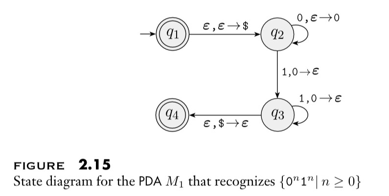
In the diagram, an arrow “${ a, b \to c }$” means the machine reads input ${ a ,}$ read-pops ${ b }$ and write-pushes ${ c }$ in that process.
We see the above PDA is ${ M = (Q, \Sigma, \Gamma, \delta, q _1, F) }$ where states are ${ Q = \lbrace q _1, q _2, q _3, q _4 \rbrace ,}$ tape symbols are ${ \Sigma = \lbrace 0,1 \rbrace, }$ stack symbols are ${ \Gamma = \lbrace 0, $ \rbrace }$ and accept states are ${ F = \lbrace q _1, q _4 \rbrace .}$

In the above example, we can think of ${ 0 }$ as being the only stack symbol, and that ${ $ }$ was used just to “signal an empty stack”. The formal definition of a PDA has no explicit mechanism to allow the PDA to test for an empty stack. Above PDA brings the same effect, by initially placing a ${ $ }$ on the stack, and then if it ever sees a ${ $ }$ again the stack is effectively empty (and the PDA reaches an accept state on read-popping the ${ $ }$).

Eg: For a string ${ w = w _1 \ldots w _n }$ in ${ \lbrace 0, 1 \rbrace ^{*} }$ it’s reverse string is ${ w ^{\mathcal{R}} = w _n \ldots w _1. }$ Here is a PDA recognizing ${ \lbrace w w ^{\mathcal{R}} : w \in \lbrace 0, 1 \rbrace ^{*} \rbrace }$ :

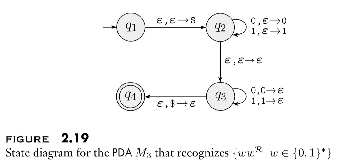
As in the above example, the ${ $ }$ technique is used to detect an empty stack. Informally the machine processes input strings as:

• Begin by pushing symbols that are read onto the stack (The “${ q _2 }$ phase”).
• At each point, nondeterministically guess the middle of the string has been reached, and change off to popping off the stack for each symbol read (i.e. switch to the “${ q _3 }$ phase”).
• If the input string ends and stack empties (i.e. stack becomes ${ $ }$) at the same time, we can reach the accept state.

Goal: Constructively show that a language is context free if and only if some pushdown automaton recognizes it.

Thm: If a language is context free, then some pushdown automaton recognizes it.
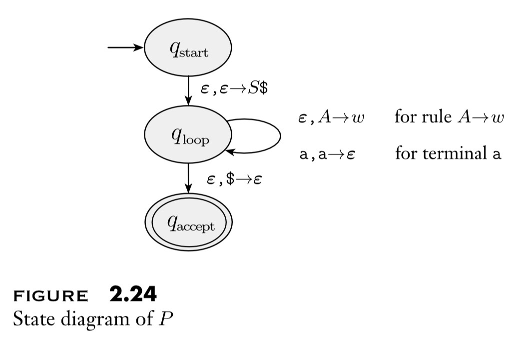
Sketch: Let ${ L }$ be a CFL. So there is a CFG ${ G }$ generating ${ L .}$ We now want a PDA ${ P }$ recognizing ${ L .}$
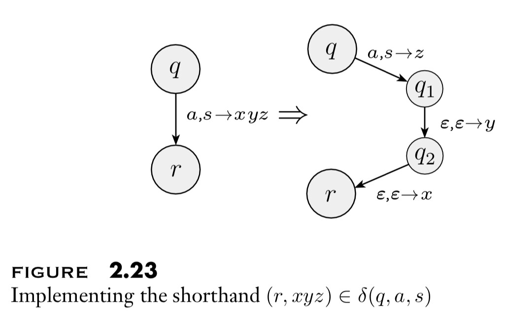
First, consider the following shorthand in drawing a PDA. In a regular PDA diagram, an arrow between states ${ q \overset{a, s \to u}{\longrightarrow} r }$ means ${ (r, u) \in \delta(q, a, s) ,}$ that is when the machine is in state ${ q }$ and follows this arrow: it reads input symbol ${ a \in \Sigma _{\varepsilon}, }$ read-pops symbol ${ s \in \Gamma _{\varepsilon} ,}$ and write-pushes symbol ${ u \in \Gamma _{\varepsilon} ,}$ moves to state ${ r.}$ In the new PDA convention, an arrow between states ${ q \overset{a, s \to u _1 \ldots u _n}{\longrightarrow} r }$ amounts to having new states and arrows \({ q \overset{a, s \to u _n}{\longrightarrow} q _1 \overset{\varepsilon, \varepsilon \to u _{n-1}}{\longrightarrow} \ldots \longrightarrow q _{n-1} \overset{\varepsilon, \varepsilon \to u _1}{\longrightarrow} r .}\)
On starting at state ${ q }$ and following the arrow(s), the machine: reads symbol ${ a \in \Sigma _{\varepsilon} },$ read-pops ${ s \in \Gamma _{\varepsilon} ,}$ and write-pushes ${ u _1 \ldots u _n }$ onto the stack, moves to state ${ r .}$ The shorthand is described, for ${ n = 3,}$ by the following diagram.

In this shorthand, the required PDA ${ P }$ is given below.

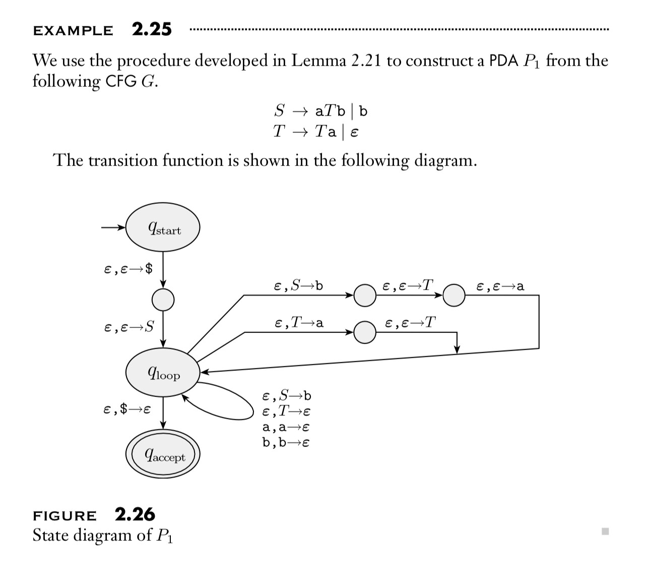
Eg: Here is an explicit example.

Thm: If a pushdown automaton recognizes a language ${ L ,}$ then ${ L }$ is context free.
(Can see Lemma 2.27 for a CFG which generates ${ L }$)

Lec-5:

(Todo: A lot)