Book: “Inference and Learning from Data” by Ali Sayed (Vols 1-3)

Python code: Link

ROUGH NOTES (!)
Updated: 3/5/24

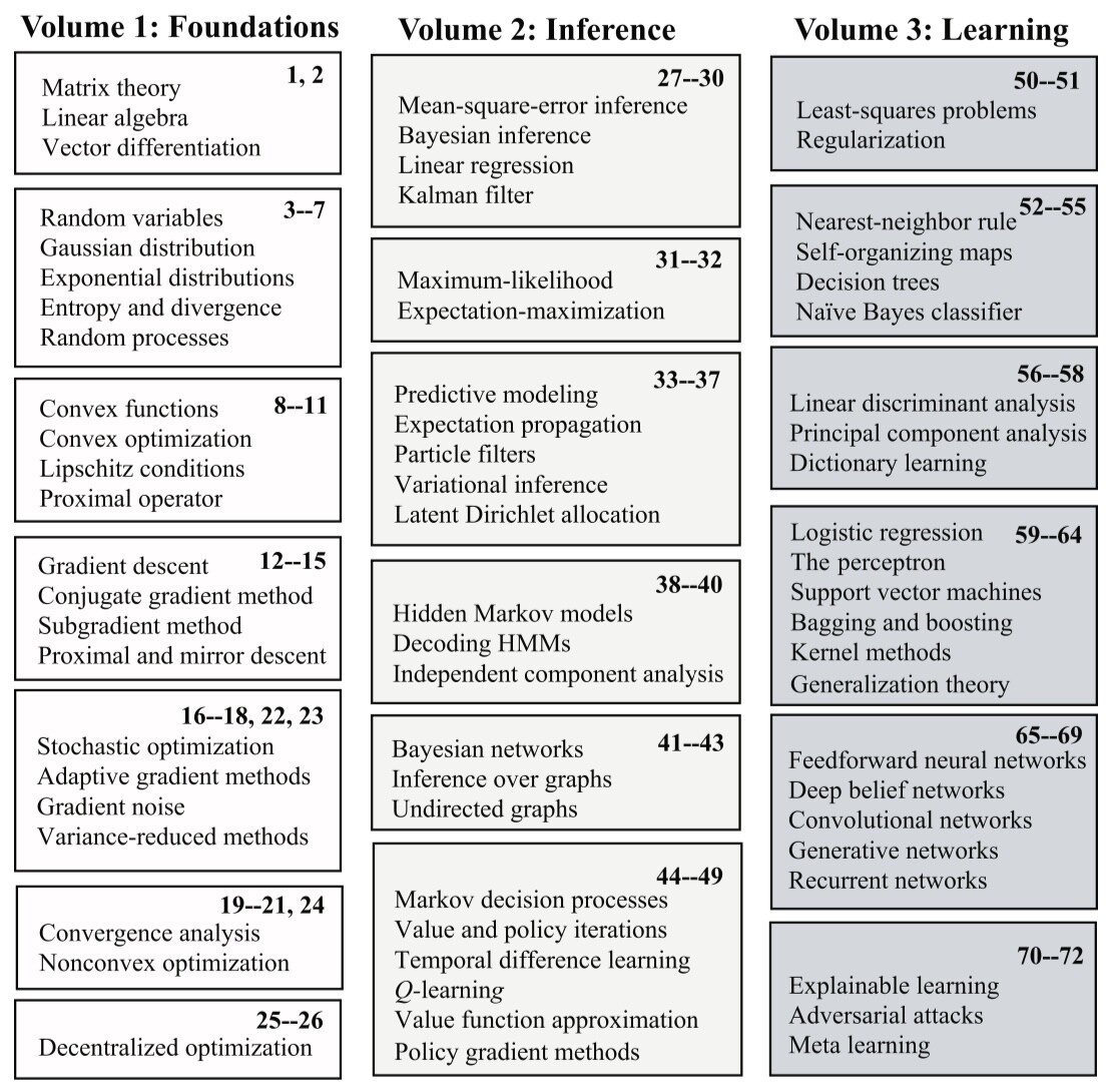
The books are organised as below.

Ch-1 Matrix Theory:
Code from booksite: None

Thm: For a real symmetric matrix ${ A \in \mathbb{R} ^{N \times N}, }$ its eigenvalues (i.e. roots of ${ f(t) = \det(tI - A) }$) are all real. (For every eigenvalue ${ \lambda \in \mathbb{R} }$ we see there is a ${ v \in \mathbb{R} ^{N}, }$ ${ v \neq 0 }$ for which ${ (\lambda I - A) v = 0 }$).
Pf: Let ${ \lambda \in \mathbb{C} }$ be an eigenvalue. So there is a ${ u \in \mathbb{C} ^N ,}$ ${ u \neq 0 }$ for which ${ A u = \lambda u .}$ Taking adjoint, since ${ A }$ is real symmetric, ${ u ^{\ast} A = \bar{\lambda} u ^{\ast}. }$ From first equation, ${ u ^{\ast} A u }$ ${ = u ^{\ast} \lambda u }$ ${ = \lambda \lVert u \rVert ^2 .}$ From the second equation, ${ u ^{\ast} A u }$ ${ = \bar{\lambda} u ^{\ast} u }$ ${ = \bar{\lambda} \lVert u \rVert ^2 .}$ So ${ \lambda = \bar{\lambda} }$ as needed.

Thm [Spectral theorem]: Every real symmetric matrix admits an orthonormal basis of eigenvectors.
Pf: The usual proof (with minor modifications for the real symmetric case). The above observation lets us pick a real eigenvalue-eigenvector pair for the first step.

Thm: Let ${ A \in \mathbb{R} ^{N \times N} }$ be real symmetric. Now its minimum and maximum eigenvalues are the minimum and maximum values of the form ${ x \mapsto x ^{T} A x }$ over on the sphere ${ \lVert x \rVert = 1 .}$ That is,

\[{ \lambda _{\text{min}} = \min _{\lVert x \rVert = 1} x ^{T} A x = \min _{x \neq 0} \frac{x ^T A x}{x ^T x} ,}\] \[{ \lambda _{\text{max}} = \max _{\lVert x \rVert = 1} x ^T A x = \max _{x \neq 0} \frac{x ^T A x}{x ^T x} .}\]

We call ${ \hat{x} ^T A \hat{x} }$ ${ = \frac{x ^T A x}{x ^T x} }$ a Rayleigh-Ritz ratio.

Pf: Since ${ A }$ is real symmetric, ${ A U = U D }$ for an orthonormal basis ${ U }$ and real diagonal matrix ${ D = \text{diag}(\lambda _1, \ldots, \lambda _N) .}$ Now

\[{ \begin{align*} \min _{\lVert x \rVert = 1} x ^T A x &= \min _{\lVert x \rVert = 1} x ^T U D U ^T x \\ &= \min _{\lVert x \rVert = 1} \sum _{n=1} ^{N} \lambda _n (U ^T x) _n ^2 \\ &= \min _{\lVert y \rVert = 1} \sum _{n=1} ^{N} \lambda _n y _n ^2 \end{align*} }\]

Over ${ \lVert y \rVert = 1 },$ we have ${ \sum _{n=1} ^N \lambda _n y _n ^2 }$ ${ \geq \lambda _{\text{min}} \sum _{n=1} ^{N} y _n ^2 }$ ${ = \lambda _{\text{min}} ,}$ with equality for eg when ${ y = e _i }$ where ${ i }$ is such that ${ \lambda _i = \lambda _{\text{min}} }.$ So

\[{ \min _{\lVert x \rVert = 1} x ^T A x = \lambda _{\text{min}} ,}\]

and similarly for maximum.

Def: Let ${ A \in \mathbb{R} ^{N \times N} }$ be real symmetric. It is called positive semidefinite (written ${ A \geq 0 }$) if ${ v ^T A v \geq 0 }$ for all ${ v \in \mathbb{R} ^N .}$ It is called positive definite (written ${ A > 0 }$) if ${ v ^T A v > 0 }$ for all ${ v \in \mathbb{R} ^N, v \neq 0 .}$
On writing ${ A U = U D }$ with ${ U }$ orthonormal and ${ D }$ diagonal, we see ${ A \geq 0 \iff \lambda _{\text{min}} \geq 0 }$ and ${ A > 0 \iff \lambda _{\text{min}} > 0 .}$

Thm [Kernel and image of ${ A ^T A }$]: For ${ A \in \mathbb{R} ^{M \times N} ,}$ spaces

\[{ \mathcal{R}(A ^T A) = \mathcal{R}(A ^T) , \quad \mathcal{N}(A ^T A ) = \mathcal{N}(A). }\]

Pf: a) Any element of ${ \mathcal{R}(A ^T A) }$ looks like ${ A ^T A v }$ and is hence in ${ \mathcal{R}(A ^T) .}$ So ${ \mathcal{R}(A ^T A ) \subseteq \mathcal{R}(A ^T) .}$
Conversely any element of ${ \mathcal{R}(A ^T) }$ looks like ${ A ^T v ,}$ and we are to show ${ A ^T v \in \mathcal{R}(A ^T A) }.$ Let ${ (A ^T A)x }$ be the projection of ${ A ^T v }$ onto ${ \mathcal{R}(A ^T A). }$ Now ${ A ^T v - (A ^T A)x }$ is orthogonal to ${ \mathcal{R}(A ^T A) .}$ Explicitly,

\[{ (A ^T (v - Ax)) ^T A^T A = 0 .}\]

The equation is ${ (v - Ax) ^T A A ^T A = 0 ,}$ and hence gives ${ (v - Ax) ^T A A ^T A {\color{red}{A ^T (v - Ax)}} = 0 }$ that is ${ (A A ^T (v-Ax)) ^T (A A ^T (v-Ax)) = 0 }$ that is

\[{ A A ^T (v - Ax) = 0 .}\]

This again gives ${ {\color{red}{(v - Ax) ^T}} A A ^T (v - Ax) = 0, }$ that is ${ (A ^T (v - Ax) ) ^T (A ^T (v - Ax)) = 0 }$ that is

\[{ A ^T (v - Ax) = 0 .}\]

So ${ A ^T v = A ^T A x \in \mathcal{R}(A ^T A), }$ as needed.

b) Any element ${ x \in \mathcal{N}(A) }$ is such that ${ Ax = 0 ,}$ and hence ${ A ^T A x = 0 }$ that is ${ x \in \mathcal{N}(A ^T A) .}$ So ${ \mathcal{N}(A) \subseteq \mathcal{N}(A ^T A). }$
Conversely any element ${ x \in \mathcal{N}(A ^T A) }$ is such that ${ A ^T A x = 0, }$ and from this we are to show ${ x \in \mathcal{N}(A) .}$ Indeed ${ {\color{red}{x ^T}} A ^T A x = 0 }$ that is ${ (Ax) ^T (Ax) = 0 }$ that is ${ Ax = 0 ,}$ as needed.

Thm: Consider the so-called normal system of equations ${ A ^T A x = A ^T b }$ for ${ A \in \mathbb{R} ^{N \times M}, b \in \mathbb{R} ^{N} }$ and variable ${ x \in \mathbb{R} ^M .}$ The following hold:

• A solution ${ x }$ always exists (since ${ A ^T b }$ ${ \in \mathcal{R}(A ^T) }$ ${ = \mathcal{R}(A ^T A) }$).
• The solution ${ x }$ is unique when ${ A ^T A }$ is invertible (when ${ \text{rk}(A ^T A) = M ,}$ i.e. when ${ \text{rk}(A) = M }$). In this case the solution is ${ x = (A ^T A) ^{-1} A ^T b .}$
• If ${ x _0 }$ is a specific solution, the full solution set is ${ x _0 + \mathcal{N}(A ^T A) }$ that is ${ x _0 + \mathcal{N}(A) .}$

Thm: Let ${ A \in \mathbb{R} ^{N \times M} ,}$ and say ${ B \in \mathbb{R} ^{N \times N} }$ is a symmetric positive definite matrix. Then

\[{ \text{rk}(A) = M \iff A ^T B A > 0 .}\]

Pf: ${ \underline{\boldsymbol{\Rightarrow}} }$ Say ${ \text{rk}(A) = M . }$ Let ${ x \in \mathbb{R} ^M , x \neq 0.}$ Since columns of ${ A }$ are linearly independent, ${ y := Ax \neq 0 .}$ So ${ x ^T (A ^T B A) x }$ ${ = y ^T B y > 0 }.$ Hence ${ A ^T B A > 0.}$
${ \underline{\boldsymbol{\Leftarrow}} }$ Say ${ A ^T B A > 0 .}$ Say to the contrary ${ \text{rk}(A) < M .}$ So there is an ${ x \in \mathbb{R} ^M, x \neq 0 }$ such that ${ Ax = 0.}$ Now ${ x ^T (A ^T B A) x }$ ${ = (Ax) ^T B (Ax) }$ ${ = 0 }$ even though ${ A ^T B A > 0 }$ and ${ x }$ is nonzero, a contradiction. So ${ \text{rk}(A) = M .}$

Schur complements:

Consider a block matrix

\[{ S = \begin{pmatrix} A &B \\ C &D \end{pmatrix} ,}\]

where ${ A }$ is ${ p \times p }$ and ${ D }$ is ${ q \times q .}$

Assuming ${ A }$ is invertible, the deletion of block ${ C }$ by elementary row operations (this doesn’t disturb block ${ A }$) looks like

\[{ \begin{align*} \begin{pmatrix} A &B \\ C &D \end{pmatrix} &\to \begin{pmatrix} I &O \\ -CA ^{-1} &I \end{pmatrix} \begin{pmatrix} A &B \\ C &D \end{pmatrix} \\ &= \begin{pmatrix} A &B \\ O &D - CA ^{-1} B \end{pmatrix}. \end{align*} }\]

Further deletion of block ${ B }$ by elementary column operations (this doesn’t disturb block ${ A }$) looks like

\[{ \begin{align*} \begin{pmatrix} A &B \\ O &D - C A ^{-1} B \end{pmatrix} &\to \begin{pmatrix} A &B \\ O &D - C A ^{-1} B \end{pmatrix} \begin{pmatrix} I &-A^{-1} B \\ O &I \end{pmatrix} \\ &= \begin{pmatrix} A &O \\ O &D - C A ^{-1} B \end{pmatrix}. \end{align*} }\]

In combined form,

\[{ \begin{pmatrix} I &O \\ -CA ^{-1} &I \end{pmatrix} \begin{pmatrix} A &B \\ C &D \end{pmatrix} \begin{pmatrix} I &-A^{-1}B \\ O &I \end{pmatrix} = \begin{pmatrix} A &O \\ O &D-CA^{-1}B \end{pmatrix} . }\]

The bottom right block

\[{ \Delta _A := D - C A ^{-1} B }\]

which remains is called Schur complement of ${ A }$ in ${ S .}$

Similarly, assuming ${ D }$ is invertible, the deletion of block ${ C }$ by elementary column operations (this doesn’t disturb block ${ D }$) and deletion of block ${ B }$ by elementary row operations (this doesn’t disturb block ${ D }$) gives

\[{ \begin{pmatrix} I &-BD^{-1} \\ O &I \end{pmatrix} \begin{pmatrix} A &B \\ C &D \end{pmatrix} \begin{pmatrix} I &O \\ -D^{-1}C &I \end{pmatrix} = \begin{pmatrix} A - BD^{-1}C &O \\ O &D \end{pmatrix}, }\]

and the top left block

\[{ \Delta _D := A - B D^{-1} C }\]

which remains is called Schur complement of ${ D }$ in ${ S .}$

Since inverses

\[{ \begin{pmatrix} I &O \\ X &I \end{pmatrix} ^{-1} = \begin{pmatrix} I &O \\ -X &I \end{pmatrix}, \quad \begin{pmatrix} I &X \\ O &I \end{pmatrix} ^{-1} = \begin{pmatrix} I &-X \\ O &I \end{pmatrix}, }\]

the above equations can be rewritten as factorisations

\[{ \begin{align*} \begin{pmatrix} A &B \\ C &D \end{pmatrix} &= \begin{pmatrix} I &O \\ CA^{-1} &I \end{pmatrix} \begin{pmatrix} A &O \\ O &\Delta _A \end{pmatrix} \begin{pmatrix} I &A^{-1}B \\ O &I \end{pmatrix} \\ &= \begin{pmatrix} I &BD^{-1} \\ O &I \end{pmatrix} \begin{pmatrix} \Delta _D &O \\ O &D \end{pmatrix} \begin{pmatrix} I &O \\ D^{-1}C &I \end{pmatrix} . \end{align*} }\]

Taking determinants gives

\[{ \det \begin{pmatrix} A &B \\ C &D \end{pmatrix} = \det(A) \det(\Delta _A) = \det(\Delta _D) \det(D) .}\]

So when ${ A }$ and ${ \Delta _A }$ are invertible, or when ${ D }$ and ${ \Delta _D }$ are invertible, the whole matrix is invertible. In this case, from the above factorisations,

\[{ \begin{align*} \begin{pmatrix} A &B \\ C &D \end{pmatrix} ^{-1} &= \begin{pmatrix} I &-A^{-1}B \\ O &I \end{pmatrix} \begin{pmatrix} A ^{-1} &O \\ O &\Delta _A ^{-1} \end{pmatrix} \begin{pmatrix} I &O \\ -CA ^{-1} &I \end{pmatrix} \\ &= \begin{pmatrix} I &O \\ -D ^{-1} C &I \end{pmatrix} \begin{pmatrix} \Delta _D ^{-1} &O \\ O &D ^{-1} \end{pmatrix} \begin{pmatrix} I &-BD^{-1} \\ O &I \end{pmatrix} , \end{align*} }\]

that is

\[{ \begin{align*} \begin{pmatrix} A &B \\ C &D \end{pmatrix} ^{-1} &= \begin{pmatrix} A^{-1} + A^{-1} B \Delta _A ^{-1} C A ^{-1} &-A^{-1} B \Delta _A ^{-1} \\ - \Delta _A ^{-1} C A ^{-1} &\Delta _A ^{-1} \end{pmatrix} \\ &= \begin{pmatrix} \Delta _D ^{-1} &-\Delta _D ^{-1} B D ^{-1} \\ - D ^{-1} C \Delta _D ^{-1} &D^{-1} + D ^{-1} C \Delta _D ^{-1} B D ^{-1} \end{pmatrix}. \end{align*} }\]

Inertia of a symmetric bilinear form:

Let ${ V }$ be an ${ n }$ dimensional real vector space and ${ \langle \cdot , \cdot \rangle : V \times V \to \mathbb{R} }$ a symmetric bilinear form.
Fixing any basis ${ \mathscr{B} = (b _1, \ldots, b _n), }$ we see the form is

\[{ \begin{align*} \langle \mathscr{B} x , \mathscr{B} y \rangle &= \left\langle \sum _{i \in [n]} b _i x _i, \sum _{j \in [n]} b _j y _j \right\rangle \\ &= \sum _{i \in [n]} x _i \left\langle b _i, \sum _{j \in [n]} b _j y _j \right\rangle \\ &= \sum _{i \in [n]} x _i \left( \sum _{j \in [n]} y _j \langle b _i, b _j \rangle \right) \\ &= x ^T (S _{\mathscr{B}}) y \end{align*} }\]

where ${ S _{\mathscr{B}} }$ is the ${ n \times n }$ symmetric matrix with entries ${ (S _{\mathscr{B}}) _{i,j} = \langle b _i, b _j \rangle .}$ We call ${ S _{\mathscr{B}} }$ the matrix of form wrt basis ${ \mathscr{B} .}$

We can first define inertia of a symmetric matrix (and then, due to Sylvester’s law of inertia, define the inertia of a symmetric bilinear form).

Def: Let ${ S \in \mathbb{R} ^{n \times n} }$ be real symmetric. So ${ SU = UD }$ with ${ U }$ orthogonal and ${ D = \text{diag}(\lambda _1, \ldots, \lambda _n) }$ real diagonal. The (multi)set of ${ \lambda _i }$s is unique, since the polynomial ${ \det(tI - S) = \det(tI - D) = \prod _{i=1} ^{n} (t - \lambda _i) .}$ We define inertia of matrix ${ S }$ as

\[{ \text{In}(S) := (I _{+} (S), I _{-} (S), I _{0} (S) ) }\]

where counts

\[{ I _{+} (S) = \# \lbrace i : \lambda _i > 0 \rbrace, }\] \[{ I _{-} (S) = \# \lbrace i : \lambda _i < 0 \rbrace , }\] \[{ I _{0} (S) = \# \lbrace i: \lambda _i = 0 \rbrace .}\]

Thm [Sylvester’s Law of Inertia]: Let ${ V }$ be an ${ n }$ dimensional real vector space and ${ \langle \cdot , \cdot \rangle : V \times V \to \mathbb{R} }$ a symmetric bilinear form. Then, for any two bases ${ \mathscr{B}, \mathscr{B} ^{’} }$ the matrix inertias

\[{ \text{In}(S _{\mathscr{B}}) = \text{In} (S _{\mathscr{B} ^{’}}) .}\]

We call this common inertia the inertia of bilinear form ${ \langle \cdot, \cdot \rangle .}$

Pf: [Ref: Meyer’s Linear Algebra book] Let ${ \mathscr{B}, \mathscr{B} ^{’} }$ be two bases of ${ V .}$ So ${ \mathscr{B} = (b _1, \ldots, b _n), }$ and ${ \mathscr{B} ^{’} = \mathscr{B} P }$ for an invertible matrix ${ P .}$

Matrices ${ S _{\mathscr{B}} , S _{\mathscr{B}P } }$ of the bilinear form are related as follows. Recalling the definition,

\[{ \langle \mathscr{B}x, \mathscr{B}y \rangle = x ^T (S _{\mathscr{B}}) y , \quad \langle \mathscr{B} P x ^{’}, \mathscr{B} P y ^{’} \rangle = (x ^{’}) ^T (S _{\mathscr{B} P }) y ^{’}. }\]

From the first equation,

\[{ \begin{align*} \langle \mathscr{B} P x ^{’} , \mathscr{B} P y ^{’} \rangle &= (P x ^{’} ) ^T S _{\mathscr{B}} (P y ^{’} ) \\ &= (x ^{’}) ^T P ^T S _{\mathscr{B}} P y ^{’} , \end{align*} }\]

and comparing this with the second equation

\[{ (x ^{’}) ^T P ^T S _{\mathscr{B}} P y ^{’} = (x ^{’}) ^T S _{\mathscr{B} P} y ^{’} \text{ for all } x ^{’}, y ^{’} \in \mathbb{R} ^n, }\]

that is

\[{ {\boxed{ S _{\mathscr{B} P} = P ^T S _{\mathscr{B}} P }} }\]

Now we are to show the matrix inertias

\[{ \text{To show: } \quad \text{In}(S _{\mathscr{B}}) = \text{In}(S _{\mathscr{B} P}) }\]

that is

\[{ \text{To show: } \quad \text{In}(S _{\mathscr{B}}) = \text{In}(P ^T S _{\mathscr{B}} P ) }\]

Say the multiset of roots of ${ \det(tI - S _{\mathscr{B}}) }$ (aka the “eigenvalues of symmetric matrix ${ S _{\mathscr{B}} }$ considered with algebraic multiplicities”) is ${ \lbrace \lambda _1, \ldots, \lambda _p, -\lambda _{p+1}, \ldots, -\lambda _{p+j}, 0, \ldots, 0 \rbrace }$ with each ${ \lambda _i > 0 .}$ So

\[{ \text{In}(S _{\mathscr{B}}) = (p, j, n - (p+j)) .}\]

Now we can write

\[{ S _{\mathscr{B}} U = U \text{diag}(\lambda _1, \ldots, \lambda _p, -\lambda _{p+1}, \ldots, -\lambda _{p+j}, 0, \ldots, 0) }\]

with ${ U }$ orthogonal. Hence

\[{ D ^T U ^T S _{\mathscr{B}} U D = \begin{pmatrix} I _p &O &O \\ O &-I _j &O \\ O &O &O _{n-(p+j)} \end{pmatrix} }\]

where ${ D = \text{diag}(\lambda _1 ^{-1/2}, \ldots, \lambda _{p+j} ^{-1/2}, 1, \ldots, 1) .}$

Similarly say the multiset of roots of ${ \det(tI - P ^T S _{\mathscr{B}} P) }$ is ${ \lbrace \mu _1, \ldots, \mu _q, -\mu _{q+1}, \ldots, - \mu _{q+k}, 0, \ldots, 0 \rbrace }$ with each ${ \mu _i > 0 .}$ Repeating the above procedure, we have

\[{ \text{In}(P ^T S _{\mathscr{B}} P) = (q, k, n-(q+k)), }\]

and

\[{ \hat{D} ^T \hat{U} ^T (P ^T S _{\mathscr{B}} P) \hat{U} \hat{D} = \begin{pmatrix} I _q &O &O \\ O &-I _k &O \\ O &O &O _{n-(q+k)} \end{pmatrix} }\]

with ${ \hat{U} }$ orthogonal and ${ \hat{D} = \text{diag}(\mu _1 ^{-1/2}, \ldots, \mu _{q+k} ^{-1/2}, 1, \ldots, 1).}$

We are to show

\[{ \text{To show: } \quad (p, j) = (q, k). }\]

From the above equations,

\[{ \underbrace{\begin{pmatrix} I _q &O &O \\ O &-I _k &O \\ O &O &O _{n-(q+k)} \end{pmatrix}} _{F} = K ^T \underbrace{\begin{pmatrix} I _p &O &O \\ O &-I _j &O \\ O &O &O _{n-(p+j)} \end{pmatrix}} _{E} K }\]

with ${ K = [K _1, \ldots, K _n] }$ invertible. Taking rank, ${ q + k = p + j .}$ So it suffices to show

\[{ \text{To show: } \quad p = q .}\]

Say ${ p > q .}$ We will arrive at a contradiction. Note for every ${ x \in \text{span}(e _1, \ldots, e _p), x \neq 0 }$ we have ${ x ^T E x > 0 }.$ Also for every ${ x = K \begin{pmatrix} 0 _{q} \\ y \end{pmatrix} , x \neq 0 }$ we have ${ x ^T E x }$ ${ = \begin{pmatrix} 0 _{q} &y ^T \end{pmatrix} \underbrace{K ^T E K} _{F} \begin{pmatrix} 0 _{q} \\ y \end{pmatrix} }$ ${ \leq 0 . }$
So to arrive at a contradiction, it suffices to pick an ${ x \in \mathcal{M} \cap \mathcal{N}, x \neq 0 }$ where ${ \mathcal{M} = \text{span}(e _1, \ldots, e _p) }$ and ${ \mathcal{N} = \text{span}(K _{q+1}, \ldots, K _n) .}$ We have dimension

\[{ \begin{align*} \dim(\mathcal{M} \cap \mathcal{N}) &= \dim(\mathcal{M}) + \dim(\mathcal{N}) - \dim(\mathcal{M} + \mathcal{N}) \\ &= p + (n-q) - \dim(\mathcal{M} + \mathcal{N}) \\ &> 0 , \end{align*} }\]

so there is an ${ x \in \mathcal{M} \cap \mathcal{N}, x \neq 0, }$ giving the required contradiction.

Similarly, assuming ${ p < q }$ also gives a contradiction. Hence ${ p = q ,}$ as needed. ${ \blacksquare }$

Eg [Inertia of symmetric block matrices]:
Consider a real symmetric block matrix

\[{ S = \begin{pmatrix} A &B \\\ B ^T &D \end{pmatrix} , \quad \text{where } A ^T = A \text{ and } D ^T = D . }\]

Say one of ${ A, D }$ is invertible. As per the case, the Schur complement factorisation is

\[{ \begin{align*} \begin{pmatrix} A &B \\\ B ^T &D \end{pmatrix} &= \begin{pmatrix} I &O \\\ B ^T A ^{-1} &I \end{pmatrix} \begin{pmatrix} A &O \\\ O &\Delta _A \end{pmatrix} \begin{pmatrix} I &A ^{-1} B \\\ O &I \end{pmatrix} \\ &= \begin{pmatrix} I &BD ^{-1} \\\ O &I \end{pmatrix} \begin{pmatrix} \Delta _D &O \\\ O &D \end{pmatrix} \begin{pmatrix} I &O \\\ D ^{-1} B ^T &I \end{pmatrix}, \end{align*} }\]

where (symmetric) Schur complements are

\[{ \Delta _A = D - B ^T A ^{-1} B , \quad \Delta _D = A - B D ^{-1} B ^T . }\]

By inertia invariance, ${ \text{In}(M) = \text{In}(P ^T M P) }$ for symmetric ${ M }$ and invertible ${ P .}$ So,

\[{ \text{In}(S) = \text{In}\begin{pmatrix} A &O \\\ O &\Delta _A \end{pmatrix} = \text{In} \begin{pmatrix} \Delta _D &O \\\ O &D \end{pmatrix} . }\]

As a special case, when ${ A }$ is invertible (so ${ \Delta _A }$ and the first factorisation exist),

\[{ \begin{align*} S > 0 &\iff \text{all roots of } \det(tI - S) \text{ are } > 0 \\ &\iff \text{In}(S) = (n, 0, 0) \\ &\iff \text{In}\begin{pmatrix} A &O \\\ O &\Delta _A \end{pmatrix} = (n, 0, 0) \\ &\iff \text{all roots of } \det(tI - A) \det(tI - \Delta _A) \text{ are } > 0 \\ &\iff A > 0 \text{ and } \Delta _A > 0. \end{align*} }\]

Similarly when ${ D }$ is invertible,

\[{ S > 0 \iff D > 0 \text{ and } \Delta _D > 0 .}\]

Cholesky factorisation:

Consider ${ A \in \mathbb{R} ^{M \times M} }$ with ${ A > 0 }$ (here this means ${ A }$ is symmetric positive definite). We can partition it as

\[{ A = \begin{pmatrix} \alpha &b^T \\\ b &D \end{pmatrix} }\]

where ${ \alpha }$ is ${ 1 \times 1 .}$
Note ${ \alpha = e _1 ^T A e _1 > 0 .}$ So we have Schur complement factorisation

\[{ \begin{pmatrix} \alpha &b^T \\\ b &D \end{pmatrix} = \begin{pmatrix} 1 &O \\\ b/{\alpha} &I \end{pmatrix} \begin{pmatrix} \alpha &O \\\ O &\Delta _{\alpha} \end{pmatrix} \begin{pmatrix} 1 &b^T/{\alpha} \\\ 0 &I \end{pmatrix} }\]

where ${ \Delta _{\alpha} = D - bb^T / {\alpha} . }$ It looks like

\[{ A = \mathcal{L} _0 \begin{pmatrix} d(0) &O \\\ O &\Delta _0 \end{pmatrix} \mathcal{L} _0 ^T , }\]

where

\[{ \mathcal{L} _0 = \begin{pmatrix} 1 &O \\\ \text{a col.} &I \end{pmatrix} , \quad d(0) = \alpha > 0 , \quad \Delta _0 = \Delta _{\alpha} > 0 . }\]

Since ${ \Delta _0 > 0, }$ by the same procedure

\[{ \Delta _0 = L _1 \begin{pmatrix} d(1) &O \\\ O &\Delta _1 \end{pmatrix} L _1 ^T }\]

where ${ L _1 = \begin{pmatrix} 1 &O \\ \text{a col.} &I \end{pmatrix},}$ ${ d(1) > 0 , }$ ${ \Delta _1 > 0 .}$ Plugging this back in,

\[{ \begin{align*} A &= \mathcal{L} _0 \begin{pmatrix} d(0) &O \\\ O &\Delta _0 \end{pmatrix} \mathcal{L} _0 ^T \\ &= {\underbrace{\mathcal{L} _0 \begin{pmatrix} 1 &O \\\ O &L _1 \end{pmatrix}} _{\mathcal{L} _1}} \begin{pmatrix} d(0) &O &O \\\ O &d(1) &O \\\ O &O &\Delta _1 \end{pmatrix} \begin{pmatrix} 1 &O \\\ O &L _1 ^T \end{pmatrix} \mathcal{L} _0 ^T \\ &= \mathcal{L} _1 \begin{pmatrix} d(0) &O &O \\\ O &d(1) &O \\\ O &O &\Delta _1 \end{pmatrix} \mathcal{L} _1 ^T . \end{align*} }\]

Continuing so,

\[{ A = \mathcal{L} _{M -1} \text{diag} (d(0), \ldots, d(M-1)) \mathcal{L} _{M-1} ^T , }\]

where ${ \mathcal{L} _{M-1} }$ is lower triangular with diagonal entries ${ 1 ,}$ and each ${ d(m) }$ is ${ > 0 .}$

Writing ${ \bar{L} = \mathcal{L} _{M-1} \mathcal{D} }$ where ${ \mathcal{D} = \text{diag}(d(0) ^{1/2}, \ldots, d(M-1) ^{1/2}) },$ we get

\[{ A = \bar{L} \bar{L} ^ T .}\]

Had we instead begun by partitioning ${ A }$ as

\[{ A = \begin{pmatrix} B &b \\\ b^T &\beta \end{pmatrix} }\]

where ${ \beta }$ is ${ 1 \times 1 ,}$ and continued as above, we would’ve got

\[{ A = \bar{U} \bar{U} ^T }\]

where ${ \bar{U} }$ is upper triangular with positive diagonal entries.

Thm [Cholesky]: Every (symmetric) positive-definite matrix ${ A }$ admits a unique factorisation of either form ${ A = \bar{L} \bar{L} ^T = \bar{U} \bar{U} ^T, }$ where ${ \bar{L} }$ (resp. ${ \bar{U} }$) is a lower (resp. upper) triangular matrix with positive diagonal entries.

Pf: Existence is as above. We will show uniqueness of the ${ \bar{L} \bar{L} ^T }$ factorisation. Say

\[{ \bar{L _1} \bar{L _1} ^T = \bar{L _2} \bar{L _2} ^T }\]

are two Cholesky factorisations for ${ A .}$ Now

\[{ \bar{L _2} ^{-1} \bar{L _1} = \bar{L _2} ^T (\bar{L _1} ^T) ^{-1} . }\]

As inverses and products of lower triangular matrices are lower triangular, above LHS is lower triangular. Similarly above RHS is upper triangular. So both sides equal a diagonal matrix, that is

\[{ \bar{L _1} = \bar{L _2} D , \quad \bar{L _2} ^T = D \bar{L _1} ^T . }\]

We see the diagonal entries of ${ D }$ are all ${ > 0 .}$ The second equation is ${ \bar{L _2} = \bar{L _1} D ^T }$ that is ${ \bar{L _2} = \bar{L _1} D .}$ Substituting this in the first equation,

\[{ \bar{L _1} = ( \bar{L _1} D ) D , }\]

giving ${ D = I , }$ that is ${ \bar{L _1 } = \bar{L _2} }$ as needed.

QR decomposition:

Let ${ x, y \in \mathbb{R} ^N }$ be nonzero. We can try decomposing ${ x }$ as ${ x = x _{\parallel} + x _{\perp} , }$ so that ${ x _{\parallel} }$ is parallel to ${ y }$ and ${ x _{\perp} }$ perpendicular to ${ y .}$ This amounts to writing ${ x = ty + (x - ty) }$ where ${ \langle x - ty, y \rangle = 0 .}$ So ${ x = \frac{\langle x, y \rangle}{\langle y, y \rangle} y + \left( x - \frac{\langle x, y \rangle}{\langle y, y \rangle} y \right) }$ is the required decomposition. We write ${ x _{\parallel} = \text{proj} _y (x) = \frac{\langle x, y \rangle}{\langle y, y \rangle} y . }$

Consider linearly independent columns ${ A = (A _1, \ldots, A _M) \in \mathbb{R} ^{N \times M} }$ (so ${ M \leq N }$). A natural way to turn it into an orthonormal set ${ (Q _1, \ldots, Q _M) }$ is:

\[{ P _1 = A _1, \quad Q _1 := P _1 / \lVert P _1 \rVert }\] \[{ P _2 = A _2 - \text{proj} _{P _1} (A _2), \quad Q _2 := P _2 / \lVert P _2 \rVert }\] \[{ P _3 = A _3 - \text{proj} _{P _1} (A _3) - \text{proj} _{P _2} (A _3) , \quad Q _3 := P _3 / \lVert P _3 \rVert }\] \[{ \vdots }\] \[{ P _M = A _M - \sum _{i=1} ^{M-1} \text{proj} _{P _i} (A _M), \quad Q _M := P _M / \lVert P _M \rVert . }\]

Formally, we can inductively/successively verify the lists

\[{ (P _1), (P _1, P _2), \ldots, (P _1, \ldots, P _M) }\]

are each orthogonal and with all elements nonzero (hence ${ (Q _1), (Q _1, Q _2), \ldots, (Q _1, \ldots, Q _M) }$ are orthonormal).

Note each ${ A _k }$ is in ${ \text{span}(P _1, \ldots, P _k) .}$ Since each ${ A _k }$ is in ${ \text{span}(Q _1, \ldots, Q _k) ,}$ writing ${ A _k = \sum _{i=1} ^{k} \lambda _i Q _i }$ and taking ${ \langle Q _i , \cdot \rangle }$ gives the coefficients ${ \lambda _i = \langle Q _i, A _k \rangle .}$ So, as is geometrically clear, each

\[{ A _k = \sum _{i=1} ^{k} \langle Q _i, A _k \rangle Q _i .}\]

In matrix notation,

\[{ (A _1, \ldots, A _M) = (Q _1, \ldots, Q _M) \begin{pmatrix} \langle Q _1, A _1 \rangle &\langle Q _1, A _2 \rangle &\langle Q _1, A _3 \rangle &\cdots &\langle Q _1, A _M \rangle \\\ 0 &\langle Q _2, A _2 \rangle &\langle Q _2, A _3 \rangle &\cdots &\langle Q _2, A _M \rangle \\\ 0 &0 &\langle Q _3, A _3 \rangle &\cdots &\langle Q _3, A _M \rangle \\\ \vdots &\vdots &\vdots &\ddots &\vdots \\\ 0 &0 &0 &\cdots &\langle Q _M, A _M \rangle \end{pmatrix}. }\]

This is called the QR decomposition of ${ A .}$

Singular Value Decomposition:

Thm: Let ${ A \in \mathbb{R} ^{M \times N} }$ be of rank ${ r > 0 .}$ Then we can write

\[{ A [\mathscr{V} _r, \mathscr{V} _{N-r}] = [\mathscr{U} _r, \mathscr{U} _{M-r}] \begin{pmatrix} \Sigma _r &O \\\ O &O \end{pmatrix}, }\]

where ${ [\mathscr{V} _r, \mathscr{V} _{N-r}] \in \mathbb{R} ^{N \times N} }$ and ${ [\mathscr{U} _r, \mathscr{U} _{M-r}] \in \mathbb{R} ^{M \times M} }$ are orthonormal bases, and ${ \Sigma _r = \text{diag}(\sigma _1, \ldots, \sigma _r) }$ with ${ \sigma _1 \geq \ldots \geq \sigma _r > 0. }$

Pf: The usual proof (but by using spectral theorem for real symmetric matrices).

Pseudoinverses:

Consider the equation ${ Ax = b }$ where ${ A \in \mathbb{R} ^{M \times N}, b \in \mathbb{R} ^{M}. }$ We can look for an approximate solution ${ \hat{x} \in \mathbb{R} ^{N} ,}$ one for which

\[{ \lVert A \hat{x} - b \rVert = \min _{x \in \mathbb{R} ^N} \lVert A x - b \rVert .}\]

Such an ${ \hat{x} }$ need not be unique. For example when ${ M = 1 }$ and ${ b = 0 .}$

By SVD,

\[{ A \mathscr{V} = \mathscr{U} \begin{pmatrix} \Sigma _r &O \\\ O &O \end{pmatrix} }\]

where ${ \mathscr{U} \in \mathbb{R} ^{M \times M} }$ and ${ \mathscr{V} \in \mathbb{R} ^{N \times N} }$ are orthonormal bases and ${ \Sigma _r = \text{diag}(\sigma _1, \ldots, \sigma _r) }$ with ${ \sigma _1 \geq \ldots \geq \sigma _r > 0 .}$

Substituting this in ${ \lVert A x - b \rVert ^2 }$ gives

\[{ \begin{align*} \lVert Ax - b \rVert ^2 &= \left\lVert \mathscr{U} \begin{pmatrix} \Sigma _r &O \\\ O &O \end{pmatrix} \mathscr{V} ^T x - b \right\rVert ^2 \\ &= \left\lVert \mathscr{U} \left( \begin{pmatrix} \Sigma _r &O \\\ O &O \end{pmatrix} \mathscr{V} ^T x - \mathscr{U} ^T b \right) \right\rVert ^2 \\ &= \left\lVert \begin{pmatrix} \Sigma _r &O \\ O &O \end{pmatrix} \begin{pmatrix} \mathscr{V} _r ^T \\\ \mathscr{V} _{N-r} ^T \end{pmatrix} x - \begin{pmatrix} \mathscr{U} _r ^T \\\ \mathscr{U} _{M-r} ^T \end{pmatrix} b \right\rVert ^2 \\ &= \lVert \Sigma _r \mathscr{V} _r ^T x - \mathscr{U} _r ^T b \rVert ^2 + \lVert \mathscr{U} _{M - r} ^T b \rVert ^2. \end{align*} }\]

The minimisers of this quantity are precisely those ${ x }$ which satisfy ${ \Sigma _r \mathscr{V} _r ^T x - \mathscr{U} _r ^T b = 0 }$ that is

\[{ \mathscr{V} _r ^T x = \Sigma _r ^{-1} \mathscr{U} _r ^T b . }\]

As ${ x = \mathscr{V} _r \Sigma _r ^{-1} \mathscr{U} _r ^T b }$ is a particular solution, the full solution set is

\[{ \begin{align*} x &\in \mathscr{V} _r \Sigma _r ^{-1} \mathscr{U} _r ^T b + \mathcal{N}(\mathscr{V} _r ^T) \\ &= \mathscr{V} _r \Sigma _r ^{-1} \mathscr{U} _r ^T b + \text{span}(\mathscr{V} _{N-r}). \end{align*} }\]

On defining pseudoinverse

\[{ A ^{\dagger} := \mathscr{V} _r \Sigma _r ^{-1} \mathscr{U} _r ^T , }\]

the set of minimisers is

\[{ \begin{align*} \text{argmin} _{x \in \mathbb{R} ^N} \lVert Ax - b \rVert &= A ^{\dagger} b + \text{span}(\mathscr{V} _{N-r}) \\ &= A ^{\dagger} b + \ker(A) . \end{align*} }\]

Note ${ A ^{\dagger} b = \mathscr{V} _r \Sigma _r ^{-1} \mathscr{U} _r ^T b }$ is in ${ \text{span}(\mathscr{V} _r) }$ and hence is orthogonal to ${ \text{span}(\mathscr{V} _{N - r}) .}$ So amongst the minimisers ${ A ^{\dagger} b + \text{span}(\mathscr{V} _{N-r}) ,}$ the minimiser with least norm is ${ A ^{\dagger} b .}$

This gives a geometric definition for the pseudoinverse: It is the matrix ${ A ^{\dagger} = (A ^{\dagger} _1, \ldots, A ^{\dagger} _M) \in \mathbb{R} ^{N \times M } }$ where each column ${ A ^{\dagger} _i }$ is the least norm element of affine subspace ${ \text{argmin} _{x \in \mathbb{R} ^N} \lVert Ax - e _i \rVert . }$

Kronecker products:
[Ref: Fuzhen Zhang’s Matrix Theory book]

Consider matrices ${ A \in \mathbb{F} ^{m \times n} }$ and ${ B \in \mathbb{F} ^{s \times t} .}$ Their Kronecker product is the ${ (ms) \times (nt) }$ matrix

\[{ A \otimes B := \begin{pmatrix} a _{11} B &a _{12} B &\cdots &a _{1n} B \\\ a _{21} B &a _{22} B &\cdots &a _{2n} B \\\ \vdots &\vdots &\ddots &\vdots \\\ a _{m1} B &a _{m2} B &\cdots &a _{mn} B \end{pmatrix} . }\]

Thm: For matrices ${ A, B, C, D}$ (of appropriate sizes when each statement is considered separately):

• ${ (kA) \otimes B = A \otimes (kB) = k(A \otimes B) }$ for any scalar ${ k .}$
• ${ (A + B) \otimes C = A \otimes C + B \otimes C .}$
• ${ A \otimes (B + C) = A \otimes B + A \otimes C .}$
• ${ A \otimes (B \otimes C) = (A \otimes B) \otimes C .}$
• ${ A \otimes B = O \iff A = O \text{ or } B = O .}$
• ${ (A \otimes B) ^{*} = A ^{*} \otimes B ^{*} }$ for complex matrices.
• ${ (A \otimes B) (C \otimes D) = (AC) \otimes (BD) .}$

Pf: It is by expanding using the definition.

For 2): Say ${ A, B }$ are ${ m \times n }.$ We see

\[{ \begin{align*} (A + B) \otimes C &= \begin{pmatrix} (a _{11} + b _{11})C &\cdots &(a _{1n} + b _{1n}) C \\\ \vdots &\ddots &\vdots \\\ (a _{m1} + b _{m1}) C &\cdots &(a _{mn} + b _{mn}) C \end{pmatrix} \\ &= \begin{pmatrix} a _{11} C &\cdots &a _{1n} C \\\ \vdots &\ddots &\vdots \\\ a _{m1} C &\cdots &a _{mn} C \end{pmatrix} + \begin{pmatrix} b _{11} C &\cdots &b _{1n} C \\\ \vdots &\ddots &\vdots \\\ b _{m1} C &\cdots &b _{mn} C \end{pmatrix} \\ &= A \otimes C + B \otimes C . \end{align*} }\]

For 4): Say ${ A }$ is ${ m \times n , }$ ${ B }$ is ${ p \times q ,}$ and ${ C }$ is ${ r \times s .}$ We see

\[{ \begin{align*} A \otimes (B \otimes C) &= \begin{pmatrix} a _{11} (B \otimes C) &\cdots &a _{1n} (B \otimes C) \\\ \vdots &\ddots &\vdots \\\ a _{m1} (B \otimes C) &\cdots &a _{mn} (B \otimes C) \end{pmatrix} \\ &= \begin{pmatrix} \begin{bmatrix} a _{11} b _{11} C &\cdots &a _{11} b _{1q} C \\\ \vdots &\ddots &\vdots \\\ a _{11} b _{p1} C &\cdots &a _{11} b _{pq} C \end{bmatrix} &\cdots &\begin{bmatrix} a _{1n} b _{11} C &\cdots &a _{1n} b _{1q} C \\\ \vdots &\ddots &\vdots \\\ a _{1n} b _{p1} C &\cdots &a _{1n} b _{pq} C \end{bmatrix} \\\ \vdots &\ddots &\vdots \\\ \begin{bmatrix} a _{m1} b _{11} C &\cdots &a _{m1} b _{1q} C \\\ \vdots &\ddots &\vdots \\\ a _{m1} b _{p1} C &\cdots &a _{m1} b _{pq} C \end{bmatrix} &\cdots &\begin{bmatrix} a _{mn} b _{11} C &\cdots &a _{mn} b _{1q} C \\\ \vdots &\ddots &\vdots \\\ a _{mn} b _{p1} C &\cdots &a _{mn} b _{pq} C \end{bmatrix} \end{pmatrix} \\ &= \begin{pmatrix} a _{11} B &\cdots &a _{1n} B \\\ \vdots &\ddots &\vdots \\\ a _{m1} B &\cdots &a _{mn} B \end{pmatrix} \otimes C \\ &= (A \otimes B) \otimes C . \end{align*} }\]

For 5): Say ${ A }$ is ${ m \times n }$ and ${ B }$ is ${ s \times t .}$ If ${ A = O }$ or ${ B = O }$ it is clear that ${ A \otimes B = O .}$
Now suppose ${ A \otimes B = O }.$ If ${ B \neq O ,}$ since

\[{ \begin{pmatrix} a _{11} B &\cdots &a _{1n} B \\\ \vdots &\ddots &\vdots \\\ a _{m1} B &\cdots &a _{mn} B \end{pmatrix} = O }\]

it must be that ${ A = O .}$ So ${ B = O , }$ or ${ A = O .}$

For 6): Say ${ A }$ is ${ m \times n }$ and ${ B }$ is ${ s \times t .}$ We see

\[{ \begin{align*} (A \otimes B) ^{*} &= \begin{pmatrix} a _{11} B &\cdots &a _{1n} B \\\ \vdots &\ddots &\vdots \\\ a _{m1} B &\cdots &a _{mn} B \end{pmatrix} ^{*} \\ &= \begin{pmatrix} \overline{a} _{11} B ^{*} &\cdots &\overline{a} _{m1} B ^{*} \\\ \vdots &\ddots &\vdots \\\ \overline{a} _{1n} B ^{*} &\cdots &\overline{a} _{mn} B ^{*} \end{pmatrix} \\ &= A ^{*} \otimes B ^{*} . \end{align*} }\]

For 7): Say ${ A }$ is ${ m \times n }$ and ${ C }$ is ${ n \times p }$ (so that ${ AC }$ is defined), and ${ B }$ is ${ q \times r }$ and ${ D }$ is ${ r \times s }$ (so that ${ BD }$ is defined). Now ${ (A \otimes B) (C \otimes D) }$ is defined as well.

Writing ${ A \otimes B }$ and ${ C \otimes D }$ as block matrices ${ A \otimes B = (a _{ij} B) _{i \in [m], j \in [n]} }$ and ${ C \otimes D = (c _{ij} D ) _{i \in [n], j \in [p]},}$ we see the ${ (i,j) }$ block of ${ (A \otimes B) (C \otimes D ) }$ is

\[{ \begin{align*} \sum _{t=1} ^{n} (a _{it} B) (c _{tj} D) &= \left( \sum _{t=1} ^{n} a _{it} c _{tj} \right) BD \\ &= (AC) _{ij} B D .\end{align*} }\]

So the full matrix is ${ (AC) \otimes (BD) .}$

Thm: Let ${ A \in \mathbb{C} ^{m \times m}, }$ ${ B \in \mathbb{C} ^{n \times n} .}$ Say the eigenvalues of ${ A }$ and ${ B ,}$ i.e. multiset of roots for ${ \det(tI-A) }$ and ${ \det(tI - B) ,}$ are ${ \lbrace \lambda _i : i \in [m] \rbrace }$ and ${ \lbrace \mu _j : j \in [n] \rbrace }$ respectively.
Then the eigenvalues of ${ A \otimes B }$ and ${ A \otimes I _n + I _m \otimes B }$ are ${ \lbrace \lambda _i \mu _j : i \in [m], j \in [n] \rbrace }$ and ${ \lbrace \lambda _i + \mu _j : i \in [m], j \in [n] \rbrace }$ respectively.

Pf: We know

\[{ \det(tI - A) = \prod _{i=1} ^{m} (t - \lambda _i), \quad \det(tI - B) = \prod _{j=1} ^{n} (t - \mu _j). }\]

By upper triangularisation,

\[{ A U = U T _A, \quad B V = V T _B }\]

with ${ U, V }$ orthonormal bases and ${ T _A, T _B}$ upper triangular. Since

\[{ \prod _{i=1} ^{m} (t - \lambda _i) = \det(tI - A) = \det(tI - T _A) = \prod _{i=1} ^{m} (t - (T _A) _{ii}) , }\]

the multiset of diagonal entries

\[{ \lbrace (T _A) _{ii} : i \in [m] \rbrace = \lbrace \lambda _i : i \in [m] \rbrace.}\]

Similarly ${ \lbrace (T _B) _{jj} : j \in [n] \rbrace = \lbrace \mu _j : j \in [n] \rbrace .}$

Note ${ U \otimes V }$ is an orthonormal basis, as

\[{ \begin{align*} (U \otimes V) ^{*} (U \otimes V) &= (U ^{*} \otimes V ^{*}) (U \otimes V) \\ &= (U ^{*} U) \otimes (V ^{*} V) \\ &= I _m \otimes I _n \\ &= I _{mn} . \end{align*} }\]

So looking at ${ A \otimes B }$ wrt orthonormal basis ${ U \otimes V ,}$

\[{ \begin{align*} (A \otimes B) (U \otimes V) &= (AU) \otimes (BV) \\ &= (UT _A) \otimes (VT _B) \\ &= (U \otimes V) (T _A \otimes T _B). \end{align*} }\]

Here

\[{ T _A \otimes T _B = \begin{pmatrix} (T _A) _{11} T _B &(T _A) _{12} T _B &\cdots &(T _A) _{1m} T _B \\\ &(T _A) _{22} T _B &\cdots &(T _A) _{2m} T _B \\\ & &\ddots &\vdots \\\ & & &(T _A) _{mm} T _B \end{pmatrix} }\]

is upper triangular, with diagonal

\[{ [(T _A) _{11} (T _B) _{jj}] _{1 \leq j \leq n} \, ; \, \ldots \, ; \, [(T _A) _{mm} (T _B) _{jj}] _{1 \leq j \leq n} }\]

which as a multiset is ${ \lbrace \lambda _i \mu _j : i \in [m], j \in [n] \rbrace .}$

Hence

\[{\begin{align*} \det(tI - A \otimes B) &= \det(tI - T _A \otimes T _B) \\ &= \prod _{k=1} ^{mn} (t - (T _ A \otimes T _ B) _{kk}) \\ &= \prod _{i=1} ^{m} \prod _{j=1} ^{n} (t - \lambda _i \mu _j), \end{align*} }\]

as needed.

Similarly, looking at ${ A \otimes I _n }$ and ${ I _m \otimes B }$ wrt orthonormal basis ${ U \otimes V, }$

\[{ \begin{align*} (A \otimes I _n) (U \otimes V) &= (AU) \otimes (I _n V) \\ &= (UT _A ) \otimes (V I _n) \\ &= (U \otimes V)(T _A \otimes I _n) \end{align*} }\]

and

\[{ \begin{align*} (I _m \otimes B) (U \otimes V) &= (I _m U) \otimes (B V) \\ &= (U I _m) \otimes (V T _B) \\ &= (U \otimes V) (I _m \otimes T _B). \end{align*} }\]

Here ${ T _A \otimes I _n }$ and ${ I _m \otimes T _B }$ are upper triangular, with diagonals

\[{ ( \underbrace{(T _A) _{11}, \ldots, (T _A) _{11}} _{n \text{ many}}; \ldots; \underbrace{(T _A) _{mm}, \ldots, (T _A) _{mm}} _{n \text{ many}} ) }\]

and

\[{ \left( (T _B) _{11}, \ldots, (T _B) _{nn}; \ldots; (T _B) _{11}, \ldots, (T _B) _{nn} \right) }\]

respectively.

Adding the above equations, we see

\[{ (A \otimes I _n + I _m \otimes B) (U \otimes V) = (U \otimes V) (T _A \otimes I _n + I _m \otimes T _B ). }\]

Also ${ T _A \otimes I _n + I _m \otimes T _B }$ is upper triangular, with diagonal

\[{ [(T _A) _{11} + (T _B) _{jj}] _{1 \leq j \leq n} \, ; \, \ldots \, ; \, [(T _A) _{mm} + (T _B) _{jj}] _{1 \leq j \leq n} }\]

which as a multiset is ${ \lbrace \lambda _i + \mu _j : i \in [m], j \in [n] \rbrace . }$

Hence

\[{ \begin{align*} \det(tI - (A \otimes I _n + I _m \otimes B)) &= \det(tI - (T _A \otimes I _n + I _m \otimes T _ B)) \\ &= \prod _{i=1} ^{m} \prod _{j=1} ^{n} (t - (\lambda _i + \mu _j)) , \end{align*} }\]

as needed. ${ \blacksquare }$

Obs: Setting ${ t = 0 }$ in ${ \det(tI - A \otimes B) = \prod _{i} \prod _{j} (t - \lambda _i \mu _j) }$ gives

\[{ \begin{align*} (-1) ^{mn} \det(A \otimes B) &= (-1) ^{mn} \left( \prod _{i=1} ^{m} \lambda _i \right) ^n \left( \prod _{j=1} ^{n} \mu _j \right) ^m \end{align*} }\]

that is

\[{ \det(A \otimes B) = \det(A) ^n \det(B) ^m .}\]

Def: Let ${ A \in \mathbb{F} ^{m \times n} .}$ The vectorisation of ${ A }$ is the ${ mn \times 1 }$ column obtained by stacking columns of ${ A }$ on top of one another, that is

\[{ \text{vec}(A) := (a _{11}, \ldots, a _{m1} \, ; \, \ldots \, ; \, a _{1n}, \ldots, a _{mn}) ^{T} . }\]

Thm: Let ${ A \in \mathbb{F} ^{m \times n} }$ and ${ B \in \mathbb{F} ^{p \times q} .}$ This gives a linear map ${ \sigma : \mathbb{F} ^{n \times p} \to \mathbb{F} ^{m \times q} }$ sending ${ X \mapsto \sigma(X) = AXB .}$ Now

\[{ \text{vec}(\sigma(X)) = (B ^T \otimes A) \text{vec}(X) , }\]

that is

\[{ \text{vec}(AXB) = (B ^T \otimes A) \text{vec}(X). }\]

(So the linear map ${ X \mapsto A X B },$ when inputs and outputs are viewed as vectors, is matrix multiplication by so-called ${ B ^T \otimes A }.$ This is one way to motivate the definition of the Kronecker product.)

Pf: We see

\[{ \begin{align*} AXB &= A(X _1, \ldots, X _p) B \\ &= (AX _1, \ldots, A X _p) B \\ &= \left( \sum _{i \in [p]} b _{i1} (AX _i) \, , \, \ldots \, , \, \sum _{i \in [p]} b _{iq} (AX _i) \right), \end{align*} }\]

so its vectorisation is

\[{ \begin{align*} \text{vec}(AXB) &= \begin{pmatrix} \sum _{i \in [p]} b _{i1} (AX _i) \\\ \vdots \\\ \sum _{i \in [p]} b _{iq} (AX _i) \end{pmatrix} \\ &= \begin{pmatrix} b _{11} A &\cdots &b _{p1} A \\\ \vdots &\ddots &\vdots \\\ b _{1q} A &\cdots &b _{pq} A \end{pmatrix} \begin{pmatrix} X _1 \\\ \vdots \\\ X _p \end{pmatrix} \\ &= (B ^T \otimes A) \text{vec}(X), \end{align*} }\]

as needed.

Matrix norms:

A matrix norm ${ \lVert \cdot \rVert }$ is a function on real matrices (for now) such that for any matrices ${ X , Y }$ of compatible dimensions and scalar ${ \alpha }$:

• ${ \lVert X \rVert \geq 0 }$
• ${ \lVert X \rVert = 0 \iff X = O }$
• ${ \lVert \alpha X \rVert = \lvert \alpha \rvert \lVert X \rVert }$
• ${ \lVert X + Y \rVert \leq \lVert X \rVert + \lVert Y \rVert }$
• ${ \lVert XY \rVert \leq \lVert X \rVert \lVert Y \rVert . }$

Recall the ${ p-}$norms on ${ \mathbb{R} ^N ,}$ and that any two norms on an ${ N }$ dimensional real vector space are equivalent.

Thm: For ${ p \geq 1 ,}$ the ${ p-}$norm on ${ \mathbb{R} ^{N} }$ is ${ \lVert x \rVert _p := \left( \sum _{i=1} ^{N} \lvert x _i \rvert ^p \right) ^{\frac{1}{p}} .}$ This gives the ${p-}$induced norm

\[{ \lVert A \rVert _p := \max _{x \neq 0} \frac{\lVert A x \rVert _p}{\lVert x \rVert _p} }\]

for matrices ${ A \in \mathbb{R} ^{M \times N} .}$ (The maximum exists because it is ${ \max }$ of ${ \lVert A x \rVert _p }$ over the compact set ${ \lbrace x \in \mathbb{R} ^N : \lVert x \rVert _p = 1 \rbrace }$).

Pf: We can for eg show triangle inequality and submultiplicativity. For ${ A, B \in \mathbb{R} ^{M \times N} }$ and ${ x \in \mathbb{R} ^N , }$

\[{ \begin{align*} \lVert (A + B) x \rVert _p &\leq \lVert Ax \rVert _p + \lVert Bx \rVert _p \\ &\leq \lVert A \rVert _p \lVert x \rVert _p + \lVert B \rVert _p \lVert x \rVert _p, \end{align*} }\]

so dividing by ${ \lVert x \rVert _p (\neq 0) }$ and taking max of LHS over ${ x \neq 0 }$ gives

\[{ \lVert A + B \rVert _p \leq \lVert A \rVert _p + \lVert B \rVert _p . }\]

For ${ A \in \mathbb{R} ^{M \times N}, }$ ${ B \in \mathbb{R} ^{N \times Q} }$ and ${ x \in \mathbb{R} ^{Q} ,}$

\[{ \lVert A (Bx) \rVert _p \leq \lVert A \rVert _p \lVert Bx \rVert _p \leq \lVert A \rVert _p \lVert B \rVert _p \lVert x \rVert _p, }\]

so dividing by ${ \lVert x \rVert _p (\neq 0) }$ and taking max of LHS over ${ x \neq 0 }$ gives

\[{ \lVert AB \rVert _p \leq \lVert A \rVert _p \lVert B \rVert _p }\]

as needed.

We also have Frobenius norm

\[{ \lVert A \rVert _F := \lVert \text{vec}(A) \rVert _2 = \sqrt{\text{Tr} (A ^T A)} . }\]

To show this is a matrix norm, it suffices to show submultiplicativity.

For ${ A \in \mathbb{R} ^{M \times N} }$ and ${ B \in \mathbb{R} ^{N \times Q} ,}$ writing ${ B = (b _1, \ldots, b _Q) }$ we have

\[{ \begin{align*} \lVert AB \rVert _F &= \sqrt{ \lVert Ab _1 \rVert ^2 + \ldots + \lVert A b _{Q} \rVert ^2 } \\ &\leq \sqrt{ \lVert A \rVert _2 ^2 \lVert b _1 \rVert ^2 + \ldots + \lVert A \rVert _2 ^2 \lVert b _Q \rVert ^2 } \\ &= \lVert A \rVert _2 \lVert B \rVert _F, \end{align*} }\]

so it suffices to show ${ \lVert A \rVert _2 \leq \lVert A \rVert _F .}$

Indeed for ${ A \in \mathbb{R} ^{M \times N} }$ and ${ x \in \mathbb{R} ^N ,}$

\[{ \begin{align*} \lVert Ax \rVert _2 &= \lVert x _1 A _1 + \ldots + x _N A _N \rVert \\ &\leq \lvert x _1 \rvert \lVert A _1 \rVert + \ldots + \lvert x _N \rvert \lVert A _N \rVert \\ &\leq \sqrt{\lvert x _1 \rvert ^2 + \ldots + \lvert x _N \rvert ^2} \sqrt{\lVert A _1 \rVert ^2 + \ldots + \lVert A _N \rVert ^2} \\ &= \lVert x \rVert _2 \lVert A \rVert _F , \end{align*} }\]

so dividing by ${ \lVert x \rVert _2 (\neq 0 )}$ and taking max over ${ x \neq 0 }$ gives

\[{ \lVert A \rVert _2 \leq \lVert A \rVert _F }\]

as needed.

Obs: Let ${ A \in \mathbb{R} ^{M \times N}. }$ By Rayleigh-Ritz for the symmetric matrix ${ A ^T A, }$

\[{ \begin{align*} \sigma _1 ^2 &= \lambda _{\text{max}} (A ^T A) \\ &= \max _{x \neq 0} \frac{x ^T A ^T A x}{x ^T x} \\ &= \max _{x \neq 0} \frac{\lVert Ax \rVert ^2}{\lVert x \rVert ^2} \\ &= \lVert A \rVert _2 ^2 , \end{align*} }\]

that is

\[{ \lVert A \rVert _2 = \sigma _1 .}\]

We also call ${ \lVert A \rVert _2 }$ the spectral norm of ${ A .}$ Similarly, using SVD ${ A = U \Sigma V ^T ,}$

\[{ \begin{align*} \lVert A \rVert _F ^2 &= \text{Tr}(A ^T A) \\ &= \text{Tr}(V \Sigma ^T U ^T U \Sigma V ^T) \\ &= \text{Tr}(V \Sigma ^T \Sigma V ^T) \\ &= \text{Tr}(\Sigma ^T \Sigma V ^T V) \\ &= \text{Tr}(\Sigma ^T \Sigma) \\ &= \sum _{i=1} ^{r} \sigma _i ^2, \end{align*} }\]

that is Frobenius norm

\[{ \lVert A \rVert _F = \left( \sum _{i=1} ^r \sigma _i ^2 \right) ^{\frac{1}{2}} .}\]

(This gives a more natural proof of ${ \lVert A \rVert _F \geq \lVert A \rVert _2 .}$)

Thm [Eckart-Young]: Consider ${ A \in \mathbb{R} ^{m \times n} }$ of positive rank ${ r .}$ By SVD,

\[{ A [v _1, \ldots, v _n] = [u _1, \ldots, u _m] \begin{pmatrix} \Sigma _r &O \\ O &O \end{pmatrix} }\]

that is

\[{ A = U \begin{pmatrix} \Sigma _r &O \\ O &O \end{pmatrix} V ^T = \sum _{i=1} ^{r} \sigma _i u _i v _i ^ T ,}\]

for orthonormal bases ${ V = [v _1, \ldots, v _n ] }$ and ${ U = [u _1, \ldots, u _m], }$ and ${ \Sigma _r = \text{diag}(\sigma _1, \ldots, \sigma _r) }$ with ${ \sigma _1 \geq \ldots \geq \sigma _r > 0 .}$

Now for each ${ s < r ,}$

\[{ \sigma _{s+1} = \inf _{\text{rk}(B) = s} \lVert A - B \rVert _2 }\]

with a minimiser

\[{ A _s = U \begin{pmatrix} \Sigma _s &O \\ O &O \end{pmatrix} V ^T = \sum _{i=1} ^{s} \sigma _i u _i v _i ^T .}\]

Pf: Given the SVD of ${ A ,}$ above matrix ${ A _s }$ is a reasonable guess for a best rank ${ s }$ approximation (wrt spectral norm) of ${ A .}$

Note ${ \text{rk}(A _s) = s }$ and

\[{ \begin{align*} \lVert A - A _s \rVert _2 &= \left\lVert \sum _{i=s+1} ^{r} \sigma _i u _i v _i ^T \right\rVert _2 \\ &= \left( 1 ^{\text{st}} \text{ singular value of } \sum _{i=s+1} ^{r} \sigma _i u _i v _i ^T \right) \\ &= \sigma _{s+1}. \end{align*} }\]

So it suffices to show

\[{ \text{To show: } \lVert A - B \rVert _2 \geq \sigma _{s+1} \text{ whenever } B \in \mathbb{R} ^{m \times n}, \text{rk}(B) = s. }\]

Say ${ B \in \mathbb{R} ^{m \times n} }$ with ${ \text{rk}(B) = s .}$ We have

\[{ \begin{align*} \lVert A - B \rVert _2 &= \lVert U\Sigma V ^T - B \rVert _2 \\ &= \max _{x \neq 0} \frac{\lVert (U \Sigma V ^T - B) x \rVert}{\lVert x \rVert} \\ &= \max _{x \neq 0} \frac{\lVert U (\Sigma - U ^T B V) V ^T x \rVert}{\lVert x \rVert} \\ &= \max _{x \neq 0} \frac{\lVert (\Sigma - U ^T BV) \overbrace{V ^T x} ^{y} \rVert}{\lVert x \rVert} \\ &= \max _{y \neq 0} \frac{\lVert (\Sigma - U ^T B V )y \rVert }{\lVert y \rVert} \\ &= \lVert \Sigma - U ^T B V \rVert _2 . \end{align*} }\]

So it suffices to show ${ \lVert \Sigma - U ^T B V \rVert _2 \geq \sigma _{s+1} ,}$ i.e. it suffices to pick an ${ x \in \mathbb{R} ^n , x \neq 0 }$ such that ${ \lVert ({\color{red}{\Sigma}} - {\color{blue}{U ^T B V}} ) x \rVert \geq \sigma _{s+1} \lVert x \rVert .}$

Note that for vectors of form ${ x = (x _1, \ldots, x _{s+1}, 0, \ldots, 0) ^ T, }$

\[{ \begin{align*} \lVert {\color{red}{\Sigma}} x \rVert &= \lVert (\sigma _1 x _1, \ldots, \sigma _{s+1} x _{s+1}, 0, \ldots, 0) ^T \rVert \\ &= \sqrt{\sigma _1 ^2 x _1 ^2 + \ldots + \sigma _{s+1} ^2 x _{s+1} ^2 } \\ &\geq \sigma _{s+1} \sqrt{x _1 ^2 + \ldots + x _{s+1} ^2 } \\ &= \sigma _{s+1} \lVert x \rVert . \end{align*} }\]

So it suffices to pick a vector of form ${ x = (x _1, \ldots, x _{s+1}, 0, \ldots, 0) ^T , }$ ${ x \neq 0 }$ such that ${ {\color{blue}{U ^T BV }}x = 0 }$ that is ${ BVx = 0 .}$

It suffices to pick a nonzero vector ${ x = (x _1, \ldots, x _{s+1}) ^T }$ such that ${ (B v _1, \ldots, B v _{s+1})x = 0 .}$

Indeed

\[{ \text{span}(B v _1, \ldots, B v _{s+1}) \subseteq \underbrace{\text{span}(B _1, \ldots, B _n)} _{\text{of dimension } \text{rk}(B) = s} ,}\]

so ${ (B v _1, \ldots, B v _{s+1}) }$ are linearly dependent, as needed. ${ \blacksquare }$

Dual norms:

Consider ${ \mathbb{R} ^M ,}$ with the usual inner product ${ x ^T y }$ (which induces the Euclidean norm ${ \lVert x \rVert _u }$) and a norm ${ \lVert \cdot \rVert .}$

By Cauchy-Schwarz we can bound the inner product ${ x ^T y }$ as

\[{ x ^T y \leq \lVert x \rVert _u \lVert y \rVert _u \quad \text{for all } x, y \in \mathbb{R} ^M .}\]

We can ask ourselves: Can we have a similar bound for the inner product ${ x ^T y }$ but involving the norm ${ \lVert \cdot \rVert }$?

Since

\[{ x ^T y \leq \left( \sup _{\lVert u \rVert = 1} x ^T u \right) \lVert y \rVert, }\]

we will be (kind of) done by saying

\[{ x ^T y \leq \lVert x \rVert _{\star} \lVert y \rVert \quad \text{for all } x, y \in \mathbb{R} ^M }\]

if

\[{ \lVert x \rVert _{\star} := \sup _{\lVert u \rVert = 1} x ^T u }\]

is a norm on ${ \mathbb{R} ^M .}$ To show the above ${ \lVert \cdot \rVert _{\star} }$ is a norm:

• Obs 1: ${ \lVert x \rVert _{\star} < \infty }$ for all ${ x \in \mathbb{R} ^M }$

This is true because of equivalence of ${ \lVert \cdot \rVert }$ with Euclidean norm ${ \lVert \cdot \rVert _{u} .}$ There exist ${ K, L > 0 }$ such that ${ K \lVert x \rVert _u \leq \lVert x \rVert \leq L \lVert x \rVert _u }$ for all ${ x \in \mathbb{R} ^M .}$ Now for any ${ x, y \in \mathbb{R} ^M }$ with ${ \lVert y \rVert = 1 , }$

\[{ \begin{align*} x ^T y &\leq \lVert x \rVert _u \lVert y \rVert _u \\ &\leq \lVert x \rVert _u \left( \frac{\lVert y \rVert}{K} \right) \\ &= \frac{1}{K} \lVert x \rVert _u , \end{align*} }\]

so

\[{ \lVert x \rVert _{\star} = \sup _{\lVert y \rVert = 1} x ^T y \leq \frac{1}{K} \lVert x \rVert _u < \infty . }\]

• Obs 2: ${ \lVert x \rVert _{\star} \geq 0 , }$ and ${ (\lVert x \rVert _{\star} = 0 \iff x = 0 )}$

This is true because for ${ x = 0 }$ the value is ${ \lVert x \rVert _{\star} = 0 , }$ and for ${ x \neq 0 }$ the value is ${ \lVert x \rVert _{\star} \geq x ^T \left( \frac{x}{\lVert x \rVert} \right) > 0 . }$

• Obs 3: ${ \lVert \alpha x \rVert _{\star} = \vert \alpha \vert \lVert x \rVert _{\star} }$ for all ${ x \in \mathbb{R} ^M, \alpha \in \mathbb{R} }$

This is true because if ${ \alpha \geq 0 }$

\[{ \begin{align*} \lVert \alpha x \rVert _{\star} &= \sup _{\lVert y \rVert = 1} (\alpha x) ^T y \\ &= \alpha \sup _{\lVert y \rVert = 1} x ^T y \\ &= \alpha \lVert x \rVert _{\star}, \end{align*} }\]

and if ${ \alpha < 0 }$

\[{ \begin{align*} \lVert \alpha x \rVert _{\star} &= \sup _{\lVert y \rVert = 1} (\alpha x) ^T y \\ &= \sup _{\lVert y \rVert = 1} (-\alpha) x ^T (-y) \\ &= (-\alpha) \sup _{\lVert u \rVert = 1} x ^T u \\ &= -\alpha \lVert x \rVert _{\star} . \end{align*} }\]

• Obs 4: ${ \lVert x + y \rVert _{\star} \leq \lVert x \rVert _{\star} + \lVert y \rVert _{\star} }$ for all ${ x , y \in \mathbb{R} ^M }$

This is true because

\[{ \begin{align*} \lVert x + y \rVert _{\star} &= \sup _{\lVert u \rVert = 1} (x ^T u + y ^T u) \\ &\leq \sup _{\lVert u \rVert = 1} x ^T u + \sup _{\lVert u \rVert = 1} y ^T u \\ &= \lVert x \rVert _{\star} + \lVert y \rVert _{\star} . \end{align*} }\]

• Obs: ${ \lVert x \rVert _{\star} := \sup _{\lVert y \rVert = 1} x ^T y = \sup _{\lVert y \rVert \leq 1} x ^T y }$

It is clear that ${ \sup _{\lVert y \rVert = 1} x ^T y \leq \sup _{\lVert y \rVert \leq 1} x ^T y .}$ It is left to show ${ \sup _{\lVert y \rVert \leq 1} x ^T y \leq \sup _{\lVert y \rVert = 1} x ^T y .}$ This is true because for any ${ y \neq 0 }$ in the interior ${ \lVert y \rVert < 1 }$ at which ${ x ^T (\cdot) }$ is ${ \geq 0 ,}$ the value ${ x ^T y \leq x ^T \left( \frac{y}{\lVert y \rVert} \right) \leq \sup _{\lVert u \rVert =1} x ^T u . }$

We call ${ \lVert \cdot \rVert _{\star} }$ the dual norm of ${ \lVert \cdot \rVert .}$

The above discussion can be extended to matrix norms.

Consider spaces ${ \mathbb{R} ^{M \times N}, }$ with the usual inner product ${ \text{Tr}(X ^T Y) }$ (which induces the Frobenius norm ${ \lVert \cdot \rVert _F }$) and a matrix norm ${ \lVert \cdot \rVert .}$

By Cauchy-Schwarz,

\[{ \text{Tr}(X ^T Y) \leq \lVert X \rVert _F \lVert Y \rVert _F \quad \text{for all } X, Y \in \mathbb{R} ^{M \times N} . }\]

On defining (as above) for ${ A \in \mathbb{R} ^{M \times N} }$ the quantity

\[{ \begin{align*} \lVert A \rVert _{\star} &:= \sup _{Y \in \mathbb{R} ^{M \times N}, \lVert Y \rVert = 1 } \text{Tr}(A ^T Y) \\ &= \sup _{Y \in \mathbb{R} ^{M \times N}, \lVert Y \rVert \leq 1} \text{Tr}(A ^T Y), \end{align*} }\]

we have

\[{ \text{Tr}(X ^T Y) \leq \lVert X \rVert _{\star} \lVert Y \rVert \quad \text{for all } X, Y \in \mathbb{R} ^{M \times N} .}\]

To show ${ \lVert \cdot \rVert _{\star} }$ is a matrix norm, by mimicking the above proof, it suffices to show submultiplicativity.

For convenience the following argument will only show the duals of Frobenius norm ${ \lVert \cdot \rVert _F }$ and spectral norm ${ \lVert \cdot \rVert _2 }$ are submultiplicative.

Let ${ A \in \mathbb{R} ^{M \times N}, B \in \mathbb{R} ^{N \times P} .}$ We are to show ${ \lVert AB \rVert _{\star} \leq \lVert A \rVert _{\star} \lVert B \rVert _{\star} .}$ If ${ A = O }$ or ${ B = O }$ it trivially holds, so say both ${ A, B \neq O .}$ Now

\[{ \begin{align*} \lVert AB \rVert _{\star} &= \sup \left\lbrace \text{Tr}((AB) ^T Y) : Y \in \mathbb{R} ^{M \times P}, \lVert Y \rVert \leq 1 \right\rbrace \\ &= \lVert A ^T \rVert \sup \bigg\lbrace \text{Tr} B ^T \underbrace{\left( \frac{A ^T Y}{\lVert A ^T \rVert } \right)} _{\varphi(Y)} : Y \in \mathbb{R} ^{M \times P}, \lVert Y \rVert \leq 1 \bigg\rbrace , \end{align*} }\]

and ${ \lVert \varphi (Y) \rVert \leq \lVert Y \rVert \leq 1 , }$ giving

\[{ \begin{align*} \lVert A B \rVert _{\star} &= \lVert A ^T \rVert \sup \bigg\lbrace \text{Tr} B ^T \left( \frac{A ^T Y}{\lVert A ^T \rVert } \right) : Y \in \mathbb{R} ^{M \times P}, \lVert Y \rVert \leq 1 \bigg\rbrace \\ &\leq \lVert A ^T \rVert \sup \bigg\lbrace \text{Tr} (B ^T U) : U \in \mathbb{R} ^{N \times P}, \lVert U \rVert \leq 1 \bigg\rbrace \\ &= \lVert A ^T \rVert \lVert B \rVert _{\star}. \end{align*} }\]

So it suffices to show

\[{ \text{Suffices to show: } \lVert A ^T \rVert \leq \lVert A \rVert _{\star} . }\]

Since

\[{ \begin{align*} \lVert A \rVert _{\star} &= \sup _{Y \in \mathbb{R} ^{M \times N}, \lVert Y \rVert \leq 1} \text{Tr}(A ^T Y) \\ &\geq \text{Tr} A ^T \frac{A}{\lVert A \rVert} \\ &= \frac{\lVert A \rVert _F ^2}{\lVert A \rVert}, \end{align*} }\]

it suffices to show ${ \frac{\lVert A \rVert _F ^2}{\lVert A \rVert} \geq \lVert A ^T \rVert }$ that is

\[{ \text{Suffices to show: } \lVert A \rVert _F ^2 \geq \lVert A \rVert \lVert A ^T \rVert . }\]

The inequality holds when ${ \lVert \cdot \rVert }$ is Frobenius norm or spectral norm: If ${ \lVert \cdot \rVert = \lVert \cdot \rVert _F ,}$ both LHS and RHS are ${ \sum _{i=1} ^{r} \sigma _i ^2 .}$ If ${ \lVert \cdot \rVert = \lVert \cdot \rVert _{2} , }$ LHS is ${ \sum _{i=1} ^{r} \sigma _i ^2 }$ and RHS is ${ \sigma _1 ^2 .}$

Hence the duals of Frobenius norm and spectral norm are submultiplicative.

Thm [Duals of common norms]:

• For ${ p \in (1, \infty), }$ the dual of vector norm ${ \lVert \cdot \rVert _p }$ is ${ \lVert \cdot \rVert _q ,}$ where ${ \frac{1}{p} + \frac{1}{q} = 1 . }$ Especially, the dual of Euclidean norm is itself.
• The dual of vector norm ${ \lVert \cdot \rVert _{1} }$ is ${ \lVert \cdot \rVert _{\infty} , }$ and vice versa.
• The dual of matrix Frobenius norm ${ \lVert \cdot \rVert _F }$ is itself.
• The dual of matrix spectral norm ${ \lVert \cdot \rVert _2 }$ is nuclear norm, given by

\[{ \lVert A \rVert _{\star} := \sum _{i=1} ^{r} \sigma _i . }\]

Pf: For 1): Let ${ p \in (1, \infty) }$ and ${ x \in \mathbb{R} ^M .}$ We are to study

\[{ \begin{align*} \lVert x \rVert _{\star} &= \sup _{\lVert u \rVert _p = 1} x ^T u \\ &= \sup _{y \neq 0} \frac{x ^T y}{\lVert y \rVert _p} . \end{align*} }\]

By Hölder’s inequality, ${ x ^T y \leq \lVert x \rVert _q \lVert y \rVert _p }$ for ${ \frac{1}{p} + \frac{1}{q} = 1 , }$ so ${ \lVert x \rVert _{\star} = \sup _{y \neq 0} \frac{x ^T y}{\lVert y \rVert _p} \leq \lVert x \rVert _{q}. }$ We will be done if this is an equality, so it suffices to show

\[{ \text{Suffices to show: } \exists \, y \neq 0 \text{ with } \frac{x ^T y}{\lVert y \rVert _p} = \lVert x \rVert _q . }\]

Heuristic to find such a ${ y }$: Assume for the moment all coordinates considered are positive. Now

\[{ \begin{align*} \frac{\partial}{\partial y _i} \left( \frac{x ^T y }{\lVert y \rVert _p } \right) ^p &= \frac{\partial}{\partial y _i} \frac{(\sum x _j y _j) ^p}{\sum y _j ^p } \\ &= \frac{p(\sum x _j y _j) ^{p-1} x _i (\sum y _j ^p) - (\sum x _j y _j) ^p p y _i ^{p-1} }{(\sum y _i ^p) ^2 } , \end{align*} }\]

and it vanishes when

\[{ x _i (\sum y _j ^p) = y _i ^{p-1} (\sum x _j y _j) }\]

that is

\[{ \frac{y _i ^p}{\sum _j y _j ^p} = \frac{x _i y _i}{\sum _j x _j y _j}. }\]

We want this to hold for all ${ i. }$ We can look for a power ${ \alpha }$ such that setting each ${ y _i = x _i ^{\alpha} }$ works. Substituting that each ${ y _i = x _i ^{\alpha} , }$

\[{ \text{We want: } \frac{x _i ^{\alpha p}}{\sum _j x _j ^{\alpha p} } = \frac{x _i ^{\alpha +1}}{\sum _j x _j ^{\alpha +1}} .}\]

So ${ \alpha p = \alpha + 1 }$ that is ${ \alpha = \frac{1}{p-1} }$ would work. At ${ y }$ with coordinates ${ y _i = x _i ^{\frac{1}{p-1}}, }$ the derivatives are all ${ 0 }$ (and ${ y }$ is, potentially, a maximiser). Letting ${ \frac{1}{p} + \frac{1}{q} = 1, }$ the choice of ${ y _i }$s can be written as

\[{ y _i = x _i ^{q-1} .}\]

At this ${ y }$ one can verify ${ \frac{x ^T y}{\lVert y \rVert _p } = \lVert x \rVert _q. }$ (This is one way to informally motivate Hölder’s inequality.)

EDIT (3/5/24): A better heuristic to find such a ${ y }$ is via Lagrange multipliers. For the moment say ${ x \in (0, \infty) ^M }$ and we want ${ \sup _{y \in (0, \infty) ^M, \lVert y \rVert _p = 1} x ^T y }$ (it is finite as ${ x ^T y }$ ${ \leq \lVert x \rVert _u \lVert y \rVert _u }$ ${ \leq \lVert x \rVert _u K \lVert y \rVert _p }$ ${ = K \lVert x \rVert _u }$ gives an upper bound) and a maximiser.

If ${ f : U (\subseteq \mathbb{R} ^n \text{ open}) \to \mathbb{R} }$ is differentiable, its derivative at ${ x }$ namely ${ (Df)(x) \in \mathbb{R} ^{1 \times n} }$ is also written as ${ (\nabla f) (x) }$ and is called the gradient of ${ f }$ at ${ x .}$

Recall Lagrange multipliers. Say ${ f : U (\subseteq \mathbb{R} ^n \text{ open}) \to \mathbb{R} }$ is ${ C ^1 }$ and surface ${ S := \lbrace x : x \in U, f(x) = 0 , \underbrace{\nabla f (x)} _{\text{a row}} \neq 0 \rbrace .}$ Now if ${ g : U \to \mathbb{R} }$ is differentiable and ${ P \in S }$ is a maximiser of ${ g : S \to \mathbb{R} , }$ we have ${ \nabla g (P) \parallel \nabla f (P).}$
The proof idea is: Intuitively, given any ${ x \in S }$ and ${ w \perp \underbrace{\nabla f (x) ^T } _{\text{normal to } S \text{ at } x} }$ there is a curve ${ \alpha : (-\varepsilon, \varepsilon) \to S }$ such that ${ \alpha(0) = x, }$ ${ \alpha ^{’} (0) = w .}$ (The formal proof uses inverse function theorem). Say ${ P }$ is a maximiser of ${ g : S \to \mathbb{R} .}$ Pick any ${ w \perp \underbrace{\nabla f (P) ^T} _{\text{normal to } S \text{ at } P} . }$ There is a curve in ${ S }$ say ${ \alpha : (-\varepsilon, \varepsilon) \to S }$ with ${ \alpha(0) = P , \alpha ^{’} (0) = w .}$ Note ${ (g \circ \alpha) (0) = \max _{t \in (-\varepsilon, \varepsilon)} (g \circ \alpha)(t), }$ so ${ 0 }$ is a local maximum giving ${ (g \circ \alpha) ^{’} (0) = 0 }$ that is ${ \nabla g (\alpha(0)) \cdot \alpha ^{’} (0) = 0 }$ that is ${ \nabla g (P) \cdot w = 0 }$ that is ${ w \perp \nabla g (P) ^T .}$ Since this is true for any ${ w \in \underbrace{(\nabla f (P) ^T ) ^{\perp}} _{n-1 \text{ dimensional}}, }$ we see ${ \nabla g (P) ^T }$ is perpendicular to the space ${ (\nabla f (P) ^T) ^{\perp} ,}$ that is ${ \nabla g (P) ^T \parallel \nabla f (P) ^T }$ as needed.

Apply Lagrange multipliers for ${ U = (0, \infty) ^M, }$ ${ f(y) = \sum y _i ^p - 1 }$ and ${ g(y) = x ^T y .}$ We see if ${ P }$ on the surface ${ S = \lbrace y : y \in (0, \infty) ^M, \lVert y \rVert _p = 1 \rbrace }$ is a maximiser of ${ g : S \to \mathbb{R} }$ we have ${ \nabla g (P) \parallel \nabla f (P) }$ that is ${ (x _1, \ldots, x _M) \parallel (p P _1 ^{p-1}, \ldots, p P _M ^{p-1}). }$ So any potential maximiser ${ P }$ of ${ g : S \to \mathbb{R} }$ looks like ${ P = \lambda (x _1 ^{1/(p-1)}, \ldots, x _M ^{1/(p-1)}) ^T = \lambda (x _1 ^{q-1}, \ldots, x _M ^{q-1}) ^T },$ as in the previous heuristic. The ${ \lambda }$ is determined by ${ \lVert P \rVert _p = 1 .}$

Back to the formal proof. Picking ${ y }$ such that ${ y _i = \text{sign}(x _i) \vert x _i \vert ^{q-1} ,}$ we see ${ x ^T y = \lVert x \rVert _q ^q }$ and

\[{ \begin{align*} \frac{x ^T y}{\lVert y \rVert _p} &= \frac{\lVert x \rVert _q ^q }{(\sum \vert x _i \vert ^{p(q-1)} ) ^{1/p} } \\ &= \frac{\lVert x \rVert _q ^q}{(\sum \vert x _i \vert ^q ) ^{1/p} } \\ &= \lVert x \rVert _q ^{q - q/p } \\ &= \lVert x \rVert _q, \end{align*} }\]

as needed.

For 2a): Let ${ x \in \mathbb{R} ^M .}$ We are to study

\[{ \lVert x \rVert _{\star} = \sup _{y \neq 0} \frac{x ^T y}{\lVert y \rVert _1} . }\]

For ${ y \neq 0 }$ we have

\[{ \frac{x ^T y}{\lVert y \rVert _1} = \frac{\sum x _i y _i}{\sum \vert y _i \vert} \leq \frac{\sum \vert x _i y _i \vert }{\sum \vert y _i \vert} \leq \max _{i} \vert x _i \vert = \lVert x \rVert _{\infty}. }\]

So it suffices to show

\[{ \text{Suffices to show: } \exists \, y \neq 0 \text{ with } \frac{x ^T y}{\lVert y \rVert _1} = \lVert x \rVert _{\infty}. }\]

Picking ${ y = \text{sign}(x _j) e _j }$ where ${ j }$ is such that ${ \vert x _j \vert = \max \vert x _i \vert ,}$ we see ${ x ^T y = \vert x _j \vert = \lVert x \rVert _{\infty} }$ and

\[{ \frac{x ^T y}{\lVert y \rVert _1} = \frac{\lVert x \rVert _{\infty}}{1} , }\]

as needed.

For 2b): Let ${ x \in \mathbb{R} ^M .}$ We are to study

\[{ \lVert x \rVert _{\star} = \sup _{y \neq 0} \frac{x ^T y}{\lVert y \rVert _{\infty}} . }\]

For ${ y \neq 0 }$ we have

\[{ \frac{x ^T y}{\lVert y \rVert _{\infty}} = \frac{\sum x _i y _i}{\max _{i} \vert y _i \vert} \leq \sum \vert x _i \vert = \lVert x \rVert _{1}. }\]

So it suffices to show

\[{ \text{Suffices to show: } \exists \, y \neq 0 \text{ with } \frac{x ^T y}{\lVert y \rVert _{\infty}} = \lVert x \rVert _1. }\]

If ${ x = 0 }$ any nonzero ${ y }$ would work, so say ${ x \neq 0 .}$ Picking ${ y }$ such that each ${ y _i = \text{sign}(x _i), }$ we see ${ x ^T y = \sum \vert x _i \vert = \lVert x \rVert _1 }$ and

\[{ \frac{x ^T y}{\lVert y \rVert _{\infty}} = \frac{\lVert x \rVert _1 }{1} , }\]

as needed.

For 3): Let ${ A \in \mathbb{R} ^{M \times N}. }$ Now dual of Frobenius norm, evaluated at ${ A ,}$ is

\[{ \begin{align*} \lVert A \rVert _{\star} &= \sup _{Y \in \mathbb{R} ^{M \times N}, Y \neq O} \frac{\text{Tr}(A ^T Y)}{\lVert Y \rVert _F } \\ &= \sup _{Y \in \mathbb{R} ^{M \times N}, Y \neq O} \frac{\text{vec}(A) ^T \text{vec}(Y) }{\lVert \text{vec}(Y) \rVert _2 } \\ &= \sup _{y \in \mathbb{R} ^{MN}, y \neq 0} \frac{\text{vec}(A) ^T y}{\lVert y \rVert _2} \\ &= \lVert \text{vec}(A) \rVert _2 \\ &= \lVert A \rVert _F , \end{align*} }\]

as needed.

For 4): Let ${ A \in \mathbb{R} ^{M \times N}. }$ We are to study

\[{ \lVert A \rVert _{\star} = \sup _{Y \in \mathbb{R} ^{M \times N}, \lVert Y \rVert _2 \leq 1 } \text{Tr}(A ^T Y) . }\]

If ${ A = O }$ the norm is ${ 0, }$ so say ${ A \neq O .}$ Using SVD ${ A = U \Sigma V ^T , }$

\[{ \begin{align*} \lVert A \rVert _{\star} &= \sup _{Y \in \mathbb{R} ^{M \times N}, \lVert Y \rVert _2 \leq 1 } \text{Tr}(A ^T Y) \\ &= \sup _{Y \in \mathbb{R} ^{M \times N}, \sigma _1 (Y) \leq 1} \text{Tr}(V \Sigma ^T U ^T Y) \\ &= \sup _{Y \in \mathbb{R} ^{M \times N}, \sigma _1 (Y) \leq 1} \text{Tr}(\Sigma ^T U ^T Y V ) \\ &= \sup _{Y \in \mathbb{R} ^{M \times N}, \sigma _1 (Y) \leq 1} \sum _{i=1} ^{r} \sigma _i \cdot (U ^T Y V) _{ii} \\ &= \sup _{Y \in \mathbb{R} ^{M \times N}, \sigma _1 (Y) \leq 1} \sum _{i=1} ^{r} \sigma _i \cdot U _i ^T \underbrace{(YV) _i} _{= Y V _i} . \end{align*} }\]

As each term

\[{ \begin{align*} U _i ^T Y V _i &= U _i ^T \hat{U} \hat{\Sigma} \hat{V} ^T V _i \\ &= (\hat{U} ^T U _i) ^T \hat{\Sigma} (\hat{V} ^T V _i) \\ &\leq \sup _{\lVert u \rVert = \lVert v \rVert = 1} u ^T \hat{\Sigma} v \\ &= \sup _{\lVert u \rVert = \lVert v \rVert = 1} \underbrace{\sum _{i=1} ^{\hat{r}} \hat{\sigma _i} u _i v _i} _{\text{is } \hat{\sigma _1} \text{ when } u = e _1, v = e _1} \\ &\leq \sup _{\lVert u \rVert = \lVert v \rVert = 1} \underbrace{\left( \sum _{i=1} ^{\hat{r}} \hat{\sigma _i} ^2 u _i ^2 \right) ^{1/2}} _{\leq \hat{\sigma _1} \lVert u \rVert = \hat{\sigma _1}} \underbrace{\left( \sum _{i=1} ^{\hat{r}} v _i ^2 \right) ^{1/2}} _{\leq \lVert v \rVert = 1} \\ &\leq \hat{\sigma _1} = \sigma _1 (Y), \end{align*} }\]

we have

\[{ \begin{align*} \lVert A \rVert _{\star} &= \sup _{Y \in \mathbb{R} ^{M \times N}, \sigma _1 (Y) \leq 1} \sum _{i=1} ^{r} \sigma _i \cdot U _i ^T Y V _i \\ &\leq \sup _{Y \in \mathbb{R} ^{M \times N}, \sigma _1 (Y) \leq 1} \sum _{i=1} ^{r} \sigma _i \sigma _1 (Y) \\ &\leq \sum _{i=1} ^{r} \sigma _i . \end{align*} }\]

So it suffices to show

\[{ \text{To show: } \exists \, Y \in \mathbb{R} ^{M \times N} \text{ with } \sigma _1 (Y) \leq 1, \text{Tr}(A ^T Y) = \sum _{i=1} ^{r} \sigma _i . }\]

Consider ${ Y = U I _{M \times N} V ^T , }$ where ${ I _{M \times N} }$ is the ${ M \times N }$ matrix with ${ 1 }$s on the diagonal and ${ 0 }$s everywhere else.

Now ${ \sigma _1 (Y) = 1 }$ and

\[{ \begin{align*} \text{Tr}(A ^T Y) &= \text{Tr}(V \Sigma ^T U ^T U I _{M \times N} V ^T) \\ &= \text{Tr}(V \Sigma ^T I _{M \times N} V ^T) \\ &= \text{Tr}(\Sigma ^T I _{M \times N} V ^T V) \\ &= \text{Tr}(\Sigma ^T I _{M \times N}) \\ &= \sum _{i=1} ^{r} \sigma _i, \end{align*} }\]

as needed. ${ \blacksquare }$